dat <- gsheet2tbl("https://docs.google.com/spreadsheets/d/1vYXB1Ag-ouLgo9nLIelP1V0hz-ki0f7p-aOCAkmuxKI/edit#gid=1058316481")
theme_set(theme_minimal_grid())Meta-analysis in Plant Pathology
Bibliographic info
Total number of pubs
nrow(dat)[1] 85dat |>
tabyl(article_type) article_type n percent
Original Article 79 0.92941176
Review 6 0.07058824Pubs per year
dat |>
  filter(pub_year > 2010) |>
  nrow()
[1] 73Pub type by year
p1 <- dat %>%
  tabyl(pub_year, article_type) %>%
  pivot_longer(names_to = "Type",
               values_to = "n", 2:3) %>%
  ggplot(aes(pub_year, n, fill = Type))+
 geom_col()+
  scale_x_continuous(breaks = c(1999, 2001, 2004, 2007, 2010, 2013, 2016,
                                2019, 2022))+
  theme(legend.position = "bottom",
          panel.grid.major=element_line(colour="grey94"))+
 scale_fill_viridis_d(option = "C")+
  scale_y_continuous(n.breaks = 10)+
  labs( x = "Publication year", y = "Number of publications")
p1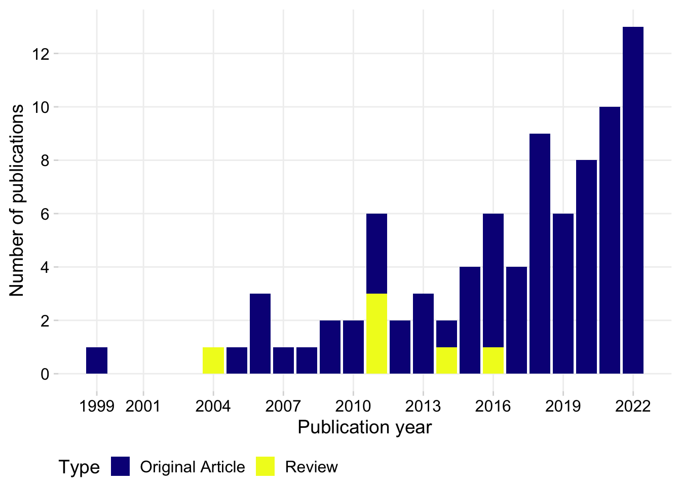
Journals
tab2 <- dat %>%
  dplyr::select(journal) %>%
   tabyl(journal) %>%
  select(-percent) |>
  arrange(-n)

tab2
journal n
Plant Disease 22
Phytopathology 21
Crop Protection 4
Plant Pathology 4
Biological Control 3
European Journal of Plant Pathology 3
Plant Health Progress 2
Summa Phytopathologica 2
African journal of agricultural research 1
Agronomy 1
Agronomy Science and Biotechnology 1
Agronomy for Sustainable Development 1
Annual Review of Phytopathology 1
Australasian Plant Pathology 1
Basic and Applied Ecology 1
BioControl 1
Biochar 1
Chemical and Biological Technologies in Agriculture 1
Ciência Rural 1
Food Security 1
HortScience 1
Journal of Fungi 1
Journal of Plant Pathology 1
Nature Earth & Environment 1
PLOS ONE 1
Physiological and Molecular Plant Pathology 1
Plant Soil 1
Plants 1
Research, Society and Development 1
Sustainability 1
The Plant Pathology Journal 1
frontiers in Molecular Biosciences 1nrow(tab2)[1] 32set.seed(3)
old_par <- par(mar = c(0, 2, 0, 0), bg = NA)
p1 + wrap_elements(panel = ~wordcloud(words = tab2$journal, freq = tab2$n, min.freq = 1, max.words=200, random.order=FALSE, rot.per=0.25, colors=brewer.pal(6, "Dark2"))) + plot_annotation(tag_levels = "A")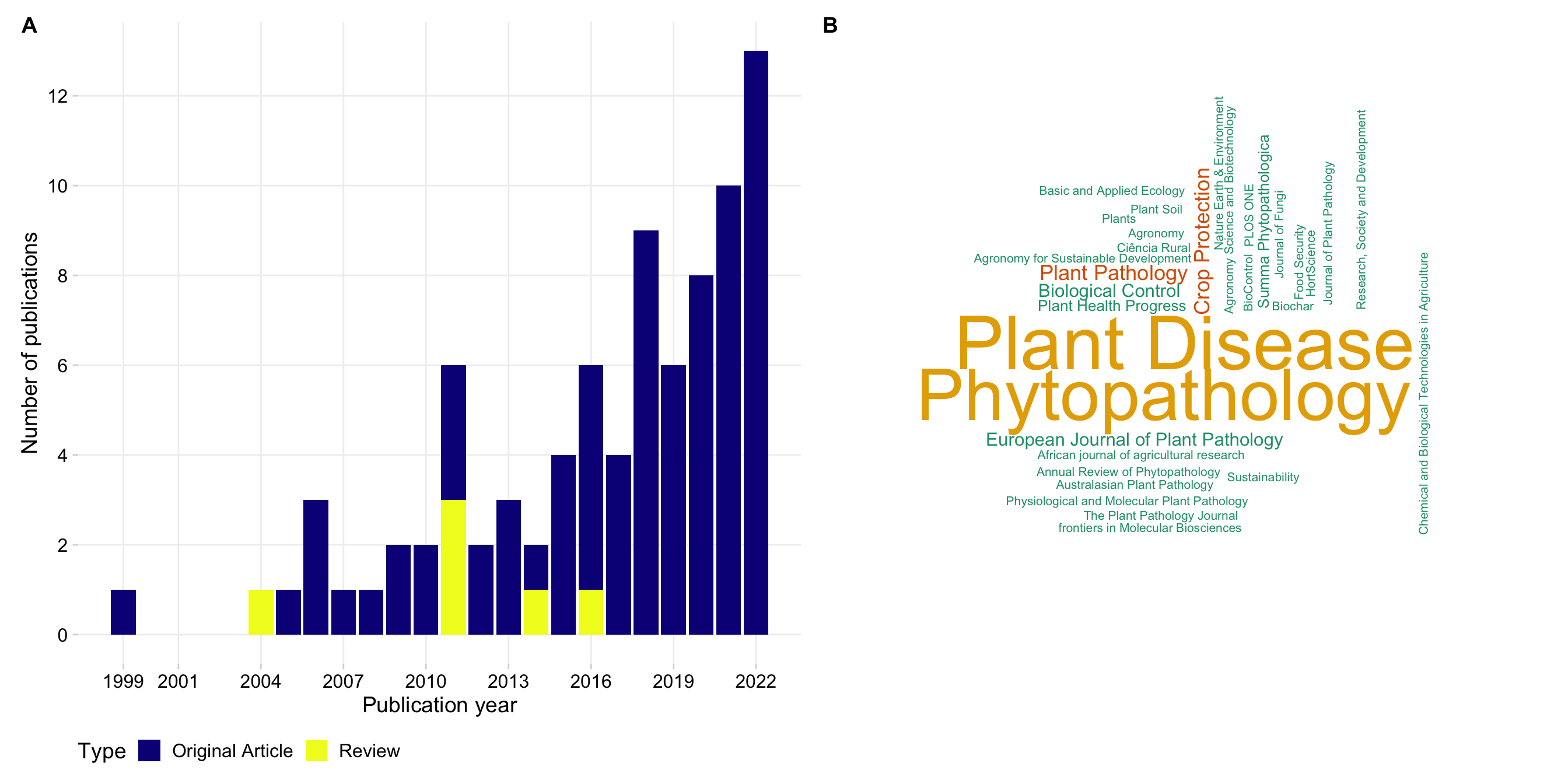
par(old_par)
ggsave("figs/figure1.png", width = 15, height = 8, bg = "white")
Number of authors per publication
dat %>%
  tabyl(n_authors)
n_authors n percent
1 1 0.01176471
2 13 0.15294118
3 14 0.16470588
4 14 0.16470588
5 15 0.17647059
6 7 0.08235294
8 3 0.03529412
10 1 0.01176471
12 2 0.02352941
13 2 0.02352941
14 1 0.01176471
15 2 0.02352941
16 1 0.01176471
18 2 0.02352941
20 1 0.01176471
21 1 0.01176471
22 1 0.01176471
23 2 0.02352941
24 1 0.01176471
32 1 0.01176471dat |>
tabyl(n_authors) |>
summary() n_authors n percent
Min. : 1.00 Min. : 1.00 Min. :0.01176
1st Qu.: 5.75 1st Qu.: 1.00 1st Qu.:0.01176
Median :13.50 Median : 2.00 Median :0.02353
Mean :13.45 Mean : 4.25 Mean :0.05000
3rd Qu.:20.25 3rd Qu.: 4.00 3rd Qu.:0.04706
Max. :32.00 Max. :15.00 Max. :0.17647 dat |>
tabyl(n_authors) |>
ggplot(aes(n_authors, n))+
geom_col(fill = "#0d0887")+
scale_y_continuous(n.breaks = 10)+
scale_x_continuous(n.breaks = 10)+
theme(legend.position = "bottom",
panel.grid.major=element_line(colour="grey94"))+
labs(y = "Frequency", x = "Number of authors per paper")
ggsave("figs/authors_paper.png", width = 5, height = 4, bg = "white")Authorship network
library(purrr)
library(purrrlyr)

authors_net <- dat_authors %>% select (2:32)
author_list <- flatten(by_row(authors_net, ..f = function(x) flatten_chr(x), .labels = FALSE))
author_list <- lapply(author_list, function(x) x[!is.na(x)])

# create the edge list
author_edge_list <- t(do.call(cbind, lapply(author_list[sapply(author_list, length) >= 2], combn, 2)))

author_edge_list[1:10, ]
[,1] [,2]
[1,] "Madden LV" "Piepho HP"
[2,] "Madden LV" "Paul PA"
[3,] "Piepho HP" "Paul PA"
[4,] "Machado FJ" "Santana FM"
[5,] "Machado FJ" "Lau D"
[6,] "Machado FJ" "Del Ponte EM"
[7,] "Santana FM" "Lau D"
[8,] "Santana FM" "Del Ponte EM"
[9,] "Lau D" "Del Ponte EM"
[10,] "Dalla Lana F" "Paul PA" Within an authorship network, co-authors (present in a same article) are linked together. Authors from these articles can be connected to authors from other articles whenever they appear together. Therefore, two articles are linked by a common author. Each author is then considered a node in the network and the connections between them are the edges or links. There are several statistics to calculate in a network analysis.
For now, let’s visualize the authorship network and also the community structure which was defined via a function that tries to find densely connected subgraphs, also called communities. We will use a random walk algorithm for determining the communities. The idea is that short random walks tend to stay in the same community. In the network below, the subgraphs are represented by the colors.
# igraph
library(igraph)
net=graph.edgelist(as.matrix(author_edge_list), directed=FALSE)

# https://www.r-econometrics.com/networks/network-summary/

#The degree of a node is the number of its connections. The degree function calculates this number for each node of a graph. The node with the highest number is the node with the highest number of connections.

hist(degree(net))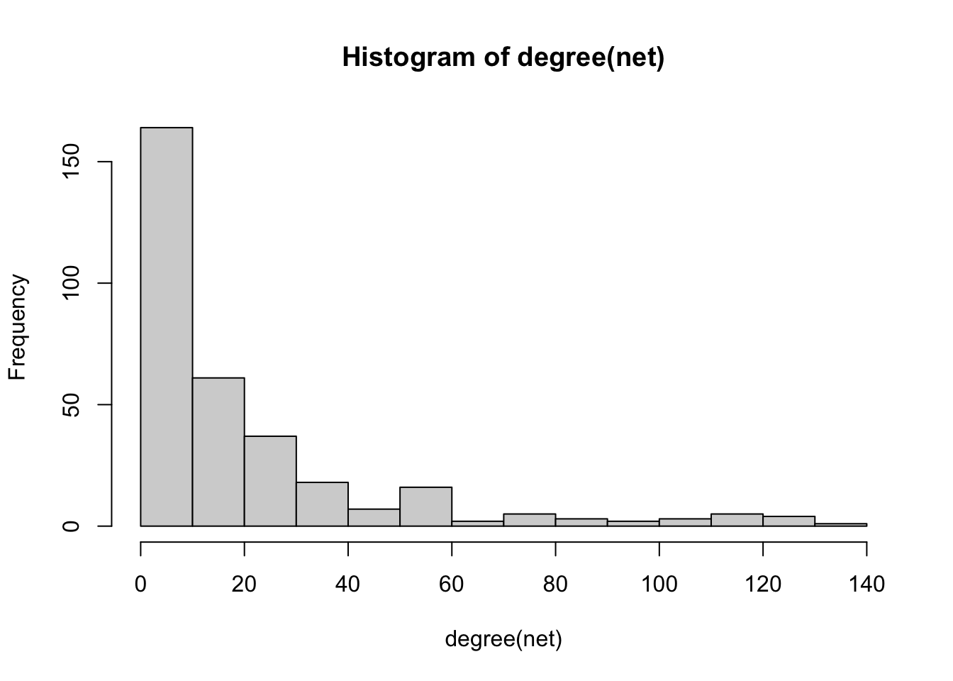
hist(log(degree(net)))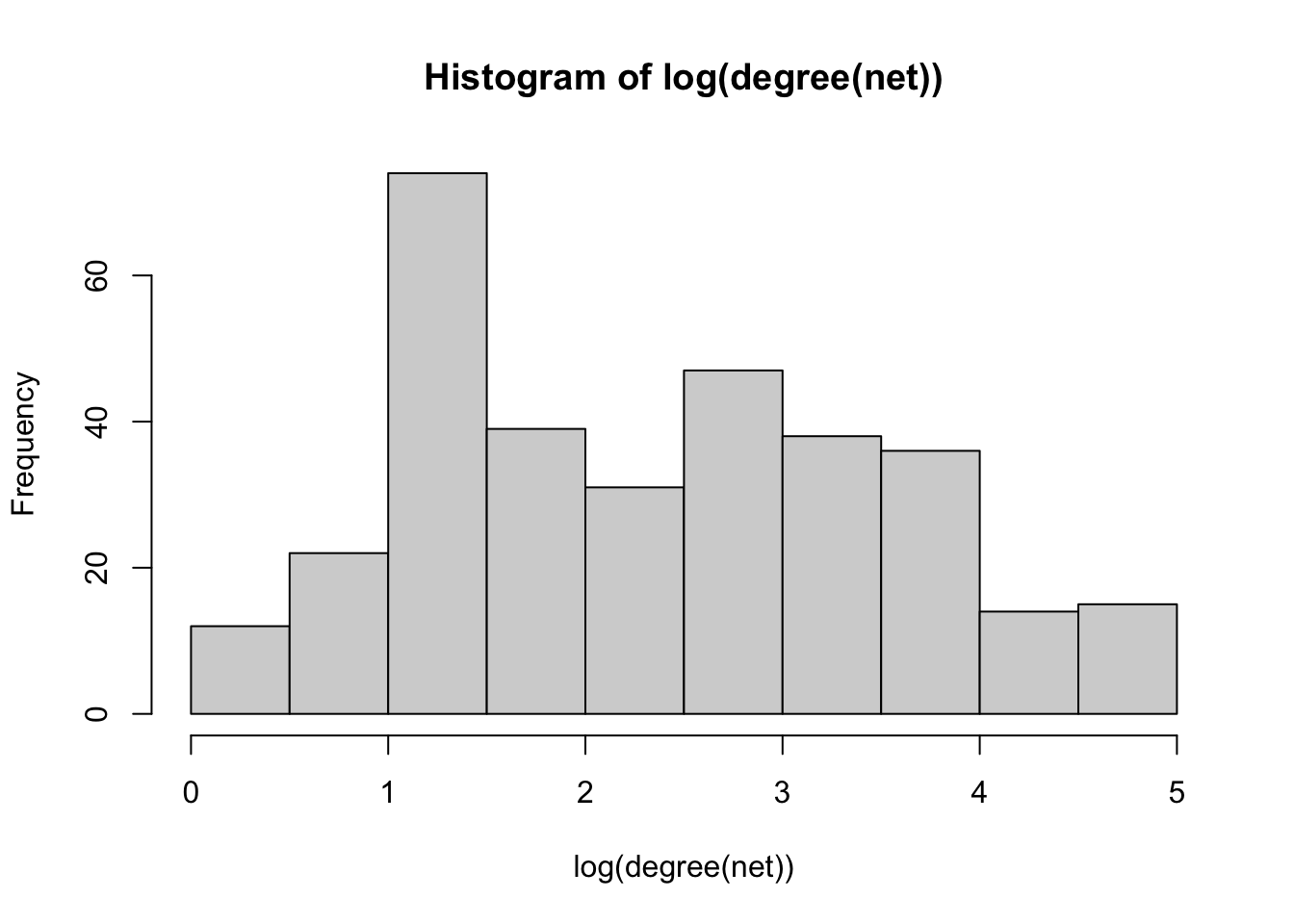
degree <- enframe(degree(net))
degree %>%  arrange(-value) |> head(10)
# A tibble: 10 × 2
name value
<chr> <dbl>
1 Godoy CV 132
2 Campos HD 124
3 Nunes J 124
4 Martins MC 124
5 Venancio WS 124
6 Paul PA 120
7 Bradley CA 116
8 Utiamada CM 115
9 Wise KA 115
10 Del Ponte EM 114#Closeness centrality describes how close a given node is to any other node. It is usually defined as the inverse of the average of the shortest path between a node and all other nodes. Therefore, shorter paths between a node and any other node in the graph imply a higher value of the ratio. In constrast to the degree of a node, which describes the number of its direct connections, its closeness provides an idea of how well a node is indirectly connected via other nodes.
close <-data.frame(round(closeness(net), 10))
close |> arrange(-round.closeness.net...10.)|> head(10) round.closeness.net...10.
Shaw DV 1
Larson KD 1
Wan JSH 1
Liew ECY 1
Toporek SM 1
Keinath AP 1
Naseri B 1
Younesi H 1
Silva RM 1
Canellas LP 1# Freeman (1977) proposes betweenness centrality as the number of shortest paths passing through a node. A higher value of a node impilies that other nodes are well connected through it.
between <- data.frame(round(betweenness(net), 1))
between |> arrange(-round.betweenness.net...1.)|> head(10) round.betweenness.net...1.
Paul PA 6625.0
Del Ponte EM 3355.8
Bradley CA 3116.9
Wise KA 2710.5
Madden LV 2606.3
Dalla Lana F 1901.8
Esker PD 1842.9
Canteri MG 1593.6
Friskop A 1407.0
Scherm H 1308.5page <- data.frame(page_rank(net)$vector)
page |> arrange(-page_rank.net..vector)|> head(10) page_rank.net..vector
Paul PA 0.011703109
Madden LV 0.011521613
Bradley CA 0.011424875
Wise KA 0.011267934
Del Ponte EM 0.009690625
Makowski D 0.009382278
Godoy CV 0.009299862
Venancio WS 0.008755985
Chilvers MI 0.008553931
Campos HD 0.008177100# Eigenvector centrality (Bonabeau, 1972) is based on the idea that the importance of a node is recusively related to the importance of the nodes pointing to it. For example, your popularity depends on the popularity of your friends, whose popularity depends on their friends etc. Therefore, this measure is also self-referential in the sense that a node’s centrality depends on the centrality of another node, whose centrality depends the first node. A higher value of eigenvector centrality implies that a node’s neighbours are more prestigious than the neighbours of other nodes.
eigen <- data.frame(round(evcent(net)$vector, 5))
eigen |> arrange(-round.evcent.net..vector..5.)|> head(10) round.evcent.net..vector..5.
Godoy CV 1.00000
Campos HD 0.97715
Nunes J 0.97715
Martins MC 0.97715
Juliatti FC 0.87839
Utiamada CM 0.82209
Meyer MC 0.80957
Venancio WS 0.79043
Furlan SH 0.77333
Carlin VJ 0.71014# Authority score is another measure of centrality initially applied to the Web. A node has high authority when it is linked by many other nodes that are linking many other nodes.
authority <- data.frame(authority_score(net)$vector)
authority |> arrange(-authority_score.net..vector)|> head(10) authority_score.net..vector
Godoy CV 1.0000000
Campos HD 0.9771517
Nunes J 0.9771517
Martins MC 0.9771517
Juliatti FC 0.8783899
Utiamada CM 0.8220877
Meyer MC 0.8095742
Venancio WS 0.7904323
Furlan SH 0.7733259
Carlin VJ 0.7101387# Collect the different centrality measures in a data frame
df <- data.frame(degree(net),
closeness(net),
betweenness(net),
eigen_centrality(net)$vector)
# Scatterplot matrix
pairs(df)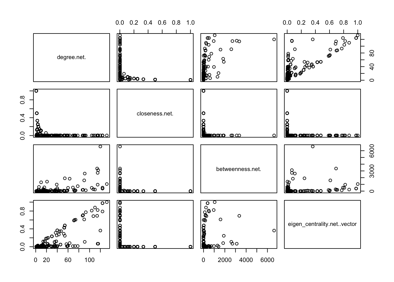
#Network properties: Let’s now try to describe what a network looks like as a whole. We can start with measures of the size of a network. diameter is the length of the longest path (in number of edges) between two nodes. We can use get_diameter to identify this path. mean_distance is the average number of edges between any two nodes in the network. We can find each of these paths between pairs of edges with distances.

diameter(net, directed = FALSE, weights = NA)
[1] 7get_diameter(net)+ 8/328 vertices, named, from 9828b31:
[1] Taylor RJ Yellareddygari SKR Friskop A Bradley CA
[5] Esker PD Scherm H Garrett KA Rosenberg MS mean_distance(net)[1] 2.773159# edge_density is the proportion of edges in the network over all possible edges that could exist.
edge_density(net)[1] 0.06369807# reciprocity measures the propensity of each edge to be a mutual edge; that is, the probability that if i is connected to j, j is also connected to i.
reciprocity(net)[1] 1# transitivity, also known as clustering coefficient, measures that probability that adjacent nodes of a network are connected. In other words, if i is connected to j, and j is connected to k, what is the probability that i is also connected to k?
transitivity(net)[1] 0.668925# Network communities - Networks often have different clusters or communities of nodes that are more densely connected to each other than to the rest of the network. Let’s cover some of the different existing methods to identify these communities. The most straightforward way to partition a network is into connected components. Each component is a group of nodes that are connected to each other, but not to the rest of the nodes. For example, this network has two components.Network graph
library(network)
library(intergraph)

# Clusters


# The walktrap algorithm finds communities through a series of short random walks. The idea is that these random walks tend to stay within the same community. The length of these random walks is 4 edges by default, but you may want to experiment with different values. The goal of this algorithm is to identify the partition that maximizes a modularity score.

wc <- cluster_walktrap(net)

#The edge-betweenness method iteratively removes edges with high betweenness, with the idea that they are likely to connect different parts of the network. Here betweenness (gatekeeping potential) applies to edges, but the intuition is the same.
eb <- cluster_edge_betweenness(net)

lec <- cluster_leading_eigen(net)

#  The label propagation method labels each node with unique labels, and then updates these labels by choosing the label assigned to the majority of their neighbors, and repeat this iteratively until each node has the most common labels among its neighbors.
cl <- cluster_label_prop(net)

# Modularity
mod <- modularity(wc)
ms <- membership(wc)

net_stat <- asNetwork(net)

png("figs/network1.png", res = 600,  width = 5000 , height = 5000, units="px")
set.seed(11)
par(mar=c(0,0,0,0))
plot.network(net_stat, vertex.cex= 0.05 + 0.25*log(graph.strength(net)),
             label =ifelse(degree(net)>50,V(net)$name, NA), label.bg = "white", label.col = "black", edge.col = "gray", label.cex = 0.6,  displaylabels = TRUE, vertex.col = membership(wc), jitter = TRUE, edge.len = 0.2, boxed.labels= T, label.border="grey", pad=5)
dev.off()
quartz_off_screen
2 library(networkD3)
#get.edgelist(net)
edge_df <- as.data.frame(get.edgelist(net))
colnames(edge_df) <- c("from", "to")
netD3 <- simpleNetwork(edge_df, zoom = T,
fontFamily = "Arial",
charge = -100,
# textColour = "black",
linkDistance = 50,
nodeColour = "black",
opacity = 0.65
)
netD3 saveNetwork(netD3, file = 'network-SAD.html')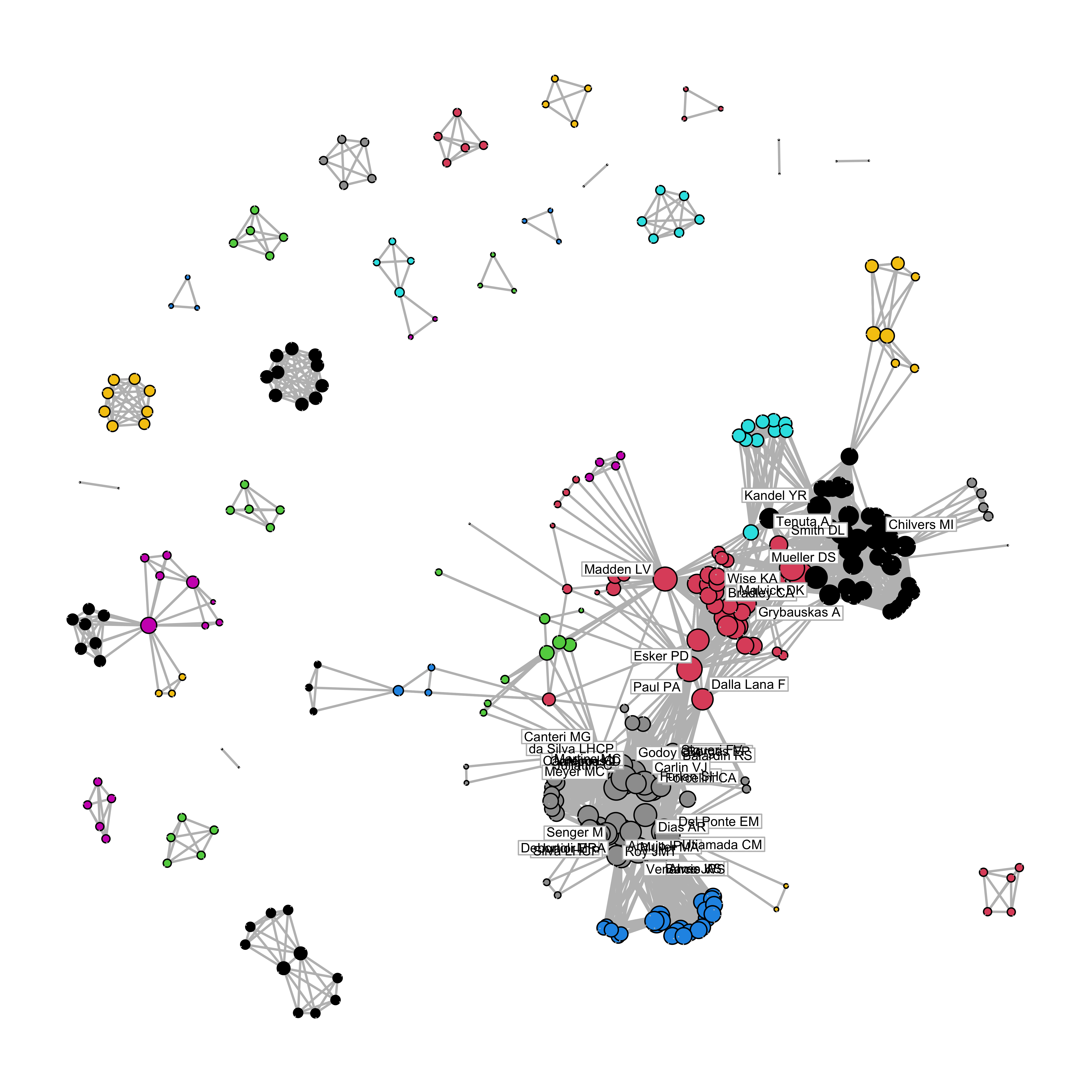
library(networkD3)


wc <- cluster_walktrap(net)
members <- membership(wc)
net2 <- igraph_to_networkD3(net, group = members)
forceNetwork(Links = net2$links, Nodes = net2$nodes,
             Source = 'source', Target = 'target',
             NodeID = 'name', Group = 'group') |>
  saveNetwork(file = 'figs/net.html')
# create a csv file of the network
write_csv(as_long_data_frame(net), file = "rede.csv")Data characteristics
Source
p2 <- dat %>%
  filter(article_type == "Original Article") %>%
  tabyl(data_source) %>%
  ggplot(aes(reorder(data_source, -n), n, fill = n))+
  geom_col(fill = "#0d0887", width = 0.56)+
  #geom_text(
   # aes(x = data_source, y = n, label = n),
    #position = position_dodge(width = 1),
    #vjust = -0.5, size = 4) +
  theme(legend.position = "bottom",
          panel.grid.major=element_line(colour="grey94"))+
scale_y_continuous(breaks = c(0, 3, 6, 9, 12, 15, 18, 21, 24, 27, 30))+
  labs(x = "Source of the data used in the analysis", y = "Number of original articles")
 p2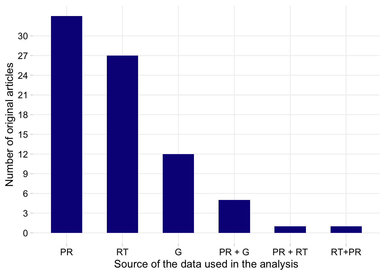
ggsave("figs/figure2.png", width =8, height = 6, bg = "white")Systematic review in PR?
dat |>
  tabyl(systematic_review, data_source)
systematic_review G PR PR + G PR + RT RT RT+PR NA_
no 11 0 0 0 27 1 0
yes 1 33 5 1 0 0 0
<NA> 0 0 0 0 0 0 6PRISM diagram?
dat |>
  tabyl(sr_flow_diag)
sr_flow_diag n percent valid_percent
no 71 0.83529412 0.8987342
yes 8 0.09411765 0.1012658
<NA> 6 0.07058824 NAStudy characteristics
Number of trials
dat |>
  count(n_trials_total) |>
  ggplot(aes(n_trials_total))+
  geom_histogram(color = "white", fill = "#0d0887")+
  labs(x = "N. of studies in the meta-analysis", y = "Frequency")+
  scale_x_continuous(n.breaks = 10)+
  theme(legend.position = "bottom",
          panel.grid.major=element_line(colour="grey94"))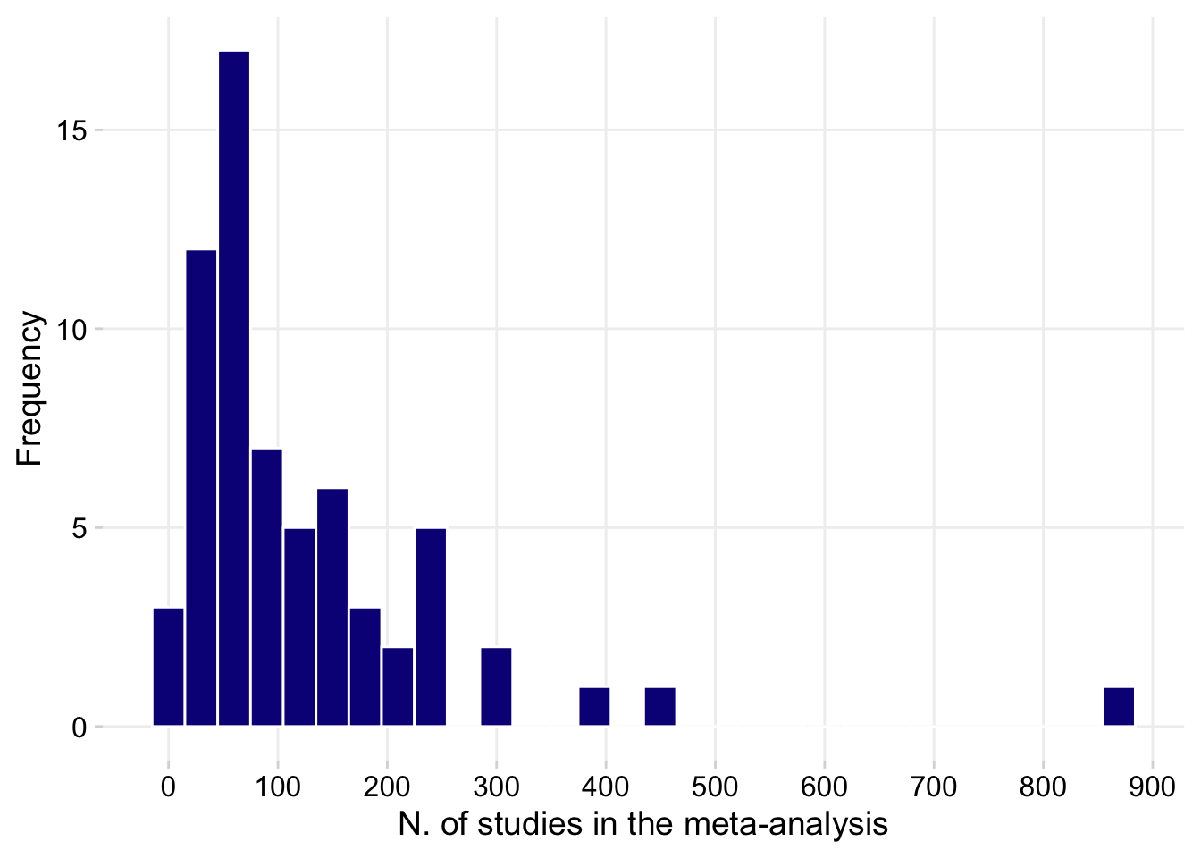
ggsave("figs/trials_study.png", width =6, height =4, bg = "white")

dat |>
  count(n_trials_total) |>
  summary()
n_trials_total n
Min. : 10 Min. :1.000
1st Qu.: 46 1st Qu.:1.000
Median : 77 Median :1.000
Mean :121 Mean :1.288
3rd Qu.:162 3rd Qu.:1.000
Max. :879 Max. :6.000
NA's :1 By objective and product type
objective <- dat %>%
  filter(article_type == "Original Article") %>%
  tabyl(objective) |>
  select(-percent)

type <- dat %>%
  filter(article_type == "Original Article") %>%
  filter(objective == "Product effects") %>%
  tabyl(product_type) |>
  select(-percent)
cbind(objective, type)
objective n product_type n
1 Dis-toxin relationship 2 BCAs 12
2 Epidemic parameter 1 Bactericides 1
3 Host effects 1 Disinfestant 3
4 Management effects 8 Fertilizer 1
5 Monocyclic component 1 Fungicide 38
6 Product and host effects 1 Fungicide+BCAs 1
7 Product effects 58 Nematicide 1
8 Yld-Dis relationship 7 Sprayers and adjuvants 1Response variables
tab <- dat %>%
  dplyr::select(response1 , response2, response3) %>%
  pivot_longer(names_to = "type", values_to = "Variable", 1:3) %>%
  select(Variable) %>%
    filter(Variable != "NA") %>%
  tabyl(Variable) %>%
  select(-percent)
nrow(tab)
[1] 38tab Variable n
100-seed weights 1
DON 6
Eggs/eggmass numbers in roots 1
RKN numbers in soil 1
Root galling 1
absolute yield 1
abundance 1
b^ 1
carpogenic germination 1
disease 1
galls index 1
incidence 15
incidence ratio 2
index 4
intensity 8
intercept 4
latent period duration 1
marketable yield 1
natural enemies 1
nematode density 1
number of cankers 1
number of eggs 1
number of galls 1
odds ratio 1
percent galled root 1
pest abundance 1
pests 1
plant biomass 2
plant growth 1
relative yield 1
sclerotia mass 1
seed germination 1
seedling emergence 1
severity 29
slope 4
test weight 1
toxin 1
yield 38library(wordcloud)
wordcloud(words = tab$Variable, freq = tab$n, min.freq = 1, max.words=200, random.order=FALSE, rot.per=0.25, colors=brewer.pal(5, "Dark2"))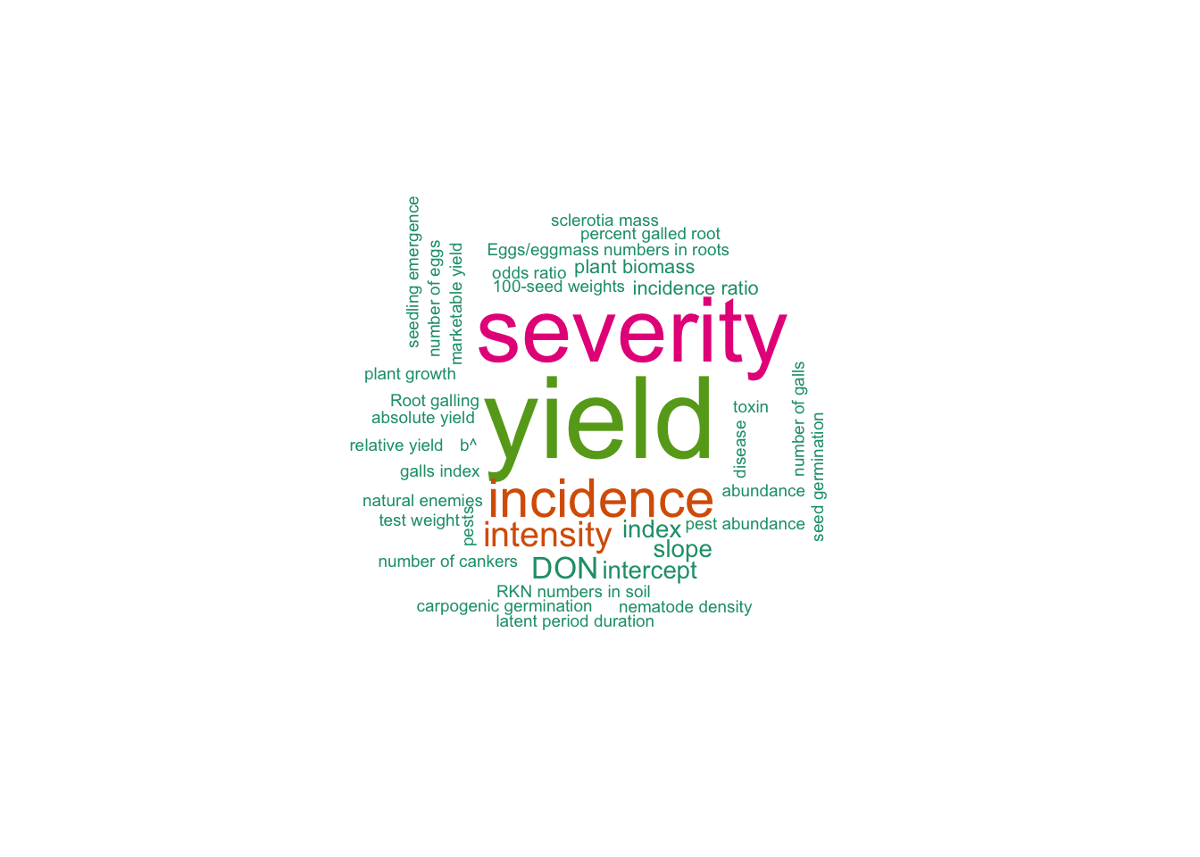
Number of responses per study
dat |>
  tabyl(n_responses)
n_responses n percent valid_percent
1 35 0.41176471 0.44871795
2 30 0.35294118 0.38461538
3 5 0.05882353 0.06410256
4 6 0.07058824 0.07692308
5 2 0.02352941 0.02564103
NA 7 0.08235294 NAMeta-analysis model characteristics
Effect sizes
es <- dat %>%
  dplyr::select(effect_size_1, effect_size_2, effect_size_3, effect_size_4, effect_size_5) %>%
  pivot_longer(names_to = "type", values_to = "value", 1:5) %>%
  select(value) %>%
    filter(value != "NA") %>%
  tabyl(value) |>
  adorn_totals()
es |>
  arrange(-n)
value n percent
Total 152 1.000000000
log ratio 36 0.236842105
means 35 0.230263158
log means 29 0.190789474
mean diff 12 0.078947368
slope 9 0.059210526
intercept 8 0.052631579
response ratio 8 0.052631579
Hedges' g 3 0.019736842
incidence ratio 3 0.019736842
odds ratio 3 0.019736842
Cohen's d 2 0.013157895
BPL b 1 0.006578947
log of d 1 0.006578947
r 1 0.006578947
risk ratio 1 0.006578947write_csv(es, "es.csv")Effect-size by common response variable
es <- dat %>%
  dplyr::select(code, effect_size_1, effect_size_2, effect_size_3, effect_size_4, effect_size_5) %>%
  pivot_longer(names_to = "type", values_to = "value", 2:6)

rv <- dat %>%
  dplyr::select(code, response1 , response2, response3, response4, response5) %>%
  pivot_longer(names_to = "type", values_to = "Variable", 2:6)

rv
# A tibble: 425 × 3
code type Variable
<dbl> <chr> <chr>
1 1 response1 <NA>
2 1 response2 <NA>
3 1 response3 <NA>
4 1 response4 <NA>
5 1 response5 <NA>
6 2 response1 severity
7 2 response2 yield
8 2 response3 <NA>
9 2 response4 <NA>
10 2 response5 <NA>
# ℹ 415 more rowsrv2 <- left_join(es, rv, by = "code") |>
select(Variable, value) |>
filter(Variable %in% c("severity", "incidence", "yield", "intensity")) |>
tabyl(value, Variable)
rv2 value incidence intensity severity yield
Cohen's d 0 1 0 1
Hedges' g 0 3 0 0
incidence ratio 3 0 0 0
intercept 0 0 4 3
log means 4 0 17 17
log of d 0 0 1 0
log ratio 14 0 18 19
mean diff 1 1 2 9
means 11 2 11 27
odds ratio 3 0 0 0
r 0 0 1 0
response ratio 0 1 2 7
risk ratio 0 1 0 0
slope 0 0 5 4
<NA> 39 31 84 118write_csv(rv2, "es2.csv")Sampling variance
dat |>
  tabyl(`Inverse variance`)
Inverse variance n percent valid_percent
no 4 0.04705882 0.05063291
not reported 4 0.04705882 0.05063291
yes 71 0.83529412 0.89873418
<NA> 6 0.07058824 NAHeterogeneity test
dat |>
  tabyl(`Heterogenity test`)
Heterogenity test n percent valid_percent
H2 and I2 1 0.01176471 0.01923077
I2 9 0.10588235 0.17307692
I2 and R2 1 0.01176471 0.01923077
LRT 8 0.09411765 0.15384615
LRT and I2 1 0.01176471 0.01923077
LRT and R2 2 0.02352941 0.03846154
Q 8 0.09411765 0.15384615
Q and I2 4 0.04705882 0.07692308
Q, H2 and I2 1 0.01176471 0.01923077
Q, I2 5 0.05882353 0.09615385
R2 2 0.02352941 0.03846154
Wald 8 0.09411765 0.15384615
Z? 1 0.01176471 0.01923077
no 1 0.01176471 0.01923077
<NA> 33 0.38823529 NAEstimator
dat |>
  tabyl(estimator)
estimator n percent valid_percent
DL 12 0.14117647 0.1518987
ML 56 0.65882353 0.7088608
Unknown 11 0.12941176 0.1392405
<NA> 6 0.07058824 NAGeneral approach
dat |>
  tabyl(ma_approach)
ma_approach n percent valid_percent
frequentist 76 0.89411765 0.96202532
frequentist and Bayesian 3 0.03529412 0.03797468
<NA> 6 0.07058824 NAMA basic model
dat |>
  tabyl(ma_model)
ma_model n percent valid_percent
MTC 23 0.27058824 0.29113924
Single treatment 53 0.62352941 0.67088608
not applicable 3 0.03529412 0.03797468
<NA> 6 0.07058824 NAdat |>
filter(ma_model == "MTC") |>
tabyl(effect_size_1, effect_size_2) effect_size_1 intercept log means log ratio mean diff means NA_
log means 0 4 0 0 8 1
log ratio 0 0 4 0 0 0
mean diff 0 0 0 1 0 1
means 1 0 0 0 1 2MA model n. of effects
dat |>
  tabyl(ma_model_2)
ma_model_2 n percent valid_percent
Kruskall-Wallis 1 0.01176471 0.01265823
fixed- and random-effects 4 0.04705882 0.05063291
fixed-effects 7 0.08235294 0.08860759
linear regression 1 0.01176471 0.01265823
mixed-effects 33 0.38823529 0.41772152
non-parametric 1 0.01176471 0.01265823
not informed 1 0.01176471 0.01265823
random- and mixed-effects 3 0.03529412 0.03797468
random-effects 27 0.31764706 0.34177215
random-effects and mixed-effects 1 0.01176471 0.01265823
<NA> 6 0.07058824 NANumber of variables
dat |>
  tabyl(ma_n_variables)
ma_n_variables n percent valid_percent
bivariate 1 0.01176471 0.01265823
univariate 78 0.91764706 0.98734177
<NA> 6 0.07058824 NAModerator analysis?
dat |>
  tabyl(moderator)
moderator n percent valid_percent
no 12 0.14117647 0.1518987
yes 67 0.78823529 0.8481013
<NA> 6 0.07058824 NAdat |>
tabyl(moderator_model) moderator_model n percent valid_percent
covariate 6 0.07058824 0.08955224
covariate and metaregression 3 0.03529412 0.04477612
metaregression 2 0.02352941 0.02985075
subgroup 31 0.36470588 0.46268657
subgroup and metaregression 23 0.27058824 0.34328358
subroup 2 0.02352941 0.02985075
<NA> 18 0.21176471 NASoftware characteristics
General software
software <- dat |>
  tabyl(general_software) |>
  arrange(general_software)

software
general_software n percent valid_percent
ARM ST 1 0.01176471 0.0125
CMA 5 0.05882353 0.0625
GENSTAT 1 0.01176471 0.0125
MetaWin 3 0.03529412 0.0375
OpenMee 1 0.01176471 0.0125
R 29 0.34117647 0.3625
SAS 31 0.36470588 0.3875
Stata 1 0.01176471 0.0125
WinBUGS 1 0.01176471 0.0125
not mentioned 2 0.02352941 0.0250
not reported 5 0.05882353 0.0625
<NA> 5 0.05882353 NAwrite_csv(software, "software.csv")dat |>
tabyl(MA_software) MA_software n percent valid_percent
CMA 4 0.04705882 0.06153846
N.M. 1 0.01176471 0.01538462
PROC GLIMMIX 8 0.09411765 0.12307692
PROC MIXED 20 0.23529412 0.30769231
PROC UNIVARIATE 1 0.01176471 0.01538462
SAS macros 2 0.02352941 0.03076923
brms 1 0.01176471 0.01538462
lme4 2 0.02352941 0.03076923
lme4 anc R2jags 1 0.01176471 0.01538462
metafor 25 0.29411765 0.38461538
<NA> 20 0.23529412 NAData summary
Results in table?
dat |>
  tabyl(res_table)
res_table n percent valid_percent
no 9 0.10588235 0.1139241
yes 70 0.82352941 0.8860759
<NA> 6 0.07058824 NAResults in plot for raw data
dat |>
  tabyl(res_plot_raw)
res_plot_raw n percent valid_percent
Yes 1 0.01176471 0.01265823
no 43 0.50588235 0.54430380
yes 35 0.41176471 0.44303797
<NA> 6 0.07058824 NAResult in forest plot
dat |>
  tabyl(res_forest)
res_forest n percent valid_percent
no 64 0.75294118 0.8101266
yes 15 0.17647059 0.1898734
<NA> 6 0.07058824 NAEconomic analysis
dat |>
  tabyl(econ_analysis)
econ_analysis n percent valid_percent
no 60 0.70588235 0.7594937
yes 19 0.22352941 0.2405063
<NA> 6 0.07058824 NA