Load packages

library(tidyverse)
library(here)
library(readxl)
library(lme4)
library(car)
library(emmeans)
library(multcomp)
library(cowplot)

South trials

dat1 <- read_excel(here("data", "data_field.xlsx"), 1) %>% 
  filter(inoculum != "test" &
           trial != "VIC2017"&
           sev != "NA" 
          #inoculum != "Fmer2x" 
         # inoculum != "Fgra2x" 
         #& sev != 0 ## remove the ears with zero severity 
         #hybrid != "supremo"
         #& hybrid != "RB9004"
         ) %>% 
  unite(ambiente, trial, hybrid, sep = ".", remove = F) %>% 
  mutate(sev = as.numeric(sev))

#dat1 %>% filter(sev == 0)
 # group_by(hybrid, rep, inoculum) %>% 
 # summarise(mean = mean(sev, na.rm = T))

Visualize

Let’s make some plots of severity data. First, let’s see differences between the hybrids across the trials

library(janitor)

## 
## Attaching package: 'janitor'

## The following objects are masked from 'package:stats':
## 
##     chisq.test, fisher.test

dat1  %>%
  tabyl(inoculum)

dat2 <- dat1 %>% 
  mutate(sev2 = asin(sqrt(sev/100)),
         sev3 = log(sev+0.5),
         sev4 = case_when(sev > 99 ~ 99,
                          sev < 1 ~ 0.1,
                          TRUE ~ sev
                          ))

dat2 %>% 
  ggplot(aes(inoculum, sev))+
  geom_boxplot(outlier.colour = NA)+
  geom_jitter(width =0.1)

dat2 %>% 
  ggplot(aes(x = sev))+
  geom_histogram()+
  facet_wrap(~ambiente)

## `stat_bin()` using `bins = 30`. Pick better value with `binwidth`.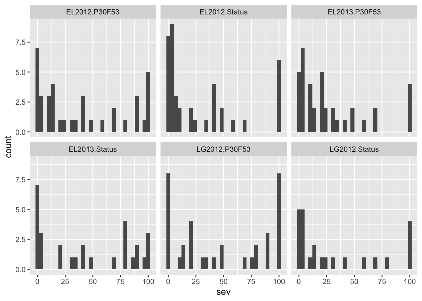

summary(dat2$sev)

##    Min. 1st Qu.  Median    Mean 3rd Qu.    Max. 
##    0.00    3.75   20.00   37.09   70.00  100.00

dat2 %>% 
  ggplot(aes(inoculum, sev, fill = inoculum))+
  geom_boxplot(outlier.colour = NA, alpha = 0.3)+
  geom_jitter(size = 2, width = 0.3, 
              shape = 16, alpha = 0.3)+
  #scale_fill_viridis_d()+
  facet_wrap(~ambiente)+
  theme_minimal_hgrid()+
  theme(legend.position = "none",axis.text.x = element_text(angle = 35, hjust = 1))+
  labs(y = "GER severity (%)", x = "Inoculation treatment")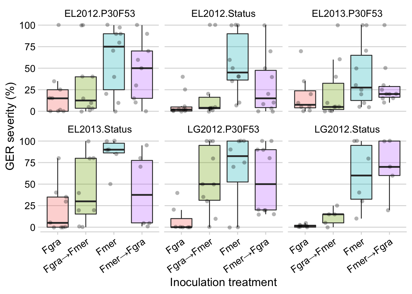

Model fit

library(glmmTMB)

med <- glmmTMB(sev4/100 ~ inoculum + (1 |trial/hybrid/rep),
                 family=beta_family(link = "logit"),
                 data = dat2)
AIC(med)

## [1] -279.1987

med0 <- lmer(logit(sev4/100) ~ inoculum + (1 | ambiente),
                                  data = dat2)

## boundary (singular) fit: see ?isSingular

med00 <- lmer(logit(sev4/100) ~ inoculum + (1 | trial/hybrid/rep),
                                  data = dat2)

## boundary (singular) fit: see ?isSingular

Anova(med00, type = "III")

icc = function(model){
    #### compute ICC
    var.components = as.data.frame(VarCorr(model))$vcov
    ICC = var.components[1]/sum(var.components)
    
    #### find out average cluster size
    id.name = names(coef(model))
    clusters = nrow(matrix(unlist((coef(model)[id.name]))))
    n = length(residuals(model))
    average.cluster.size = n/clusters
    
    #### compute design effects
    design.effect = 1+ICC*(average.cluster.size-1)
    
    #### return stuff
    list(icc=ICC, design.effect=design.effect)
    
}
icc(med00)

## $icc
## [1] 0.1339909
## 
## $design.effect
## [1] 0.9695475

as.data.frame(VarCorr(med00))

Residual

library(DHARMa)

## This is DHARMa 0.3.3.0. For overview type '?DHARMa'. For recent changes, type news(package = 'DHARMa') Note: Syntax of plotResiduals has changed in 0.3.0, see ?plotResiduals for details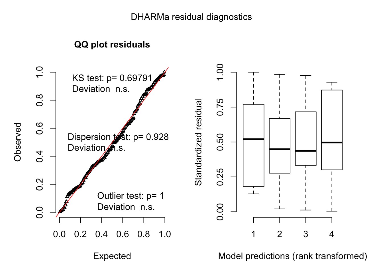

simres <- simulateResiduals(med0)
plot(simres)

Multiple comparison

medias2 <- emmeans(med0, pairwise~inoculum, type = "response")
medias2$emmeans

##  inoculum  response      SE   df lower.CL upper.CL
##  Fgra        0.0218 0.00938 64.1  0.00914   0.0509
##  Fgra→Fmer   0.1942 0.06779 57.6  0.09198   0.3646
##  Fmer        0.6768 0.09758 62.8  0.46198   0.8363
##  Fmer→Fgra   0.4110 0.10809 61.5  0.22222   0.6301
## 
## Degrees-of-freedom method: kenward-roger 
## Confidence level used: 0.95 
## Intervals are back-transformed from the logit scale

pwpp plot

library(cowplot)
p1 <- pwpp(medias2$emmeans, add.space =3, sort = F)+
  theme_minimal_grid()+
  labs(y = "")
p1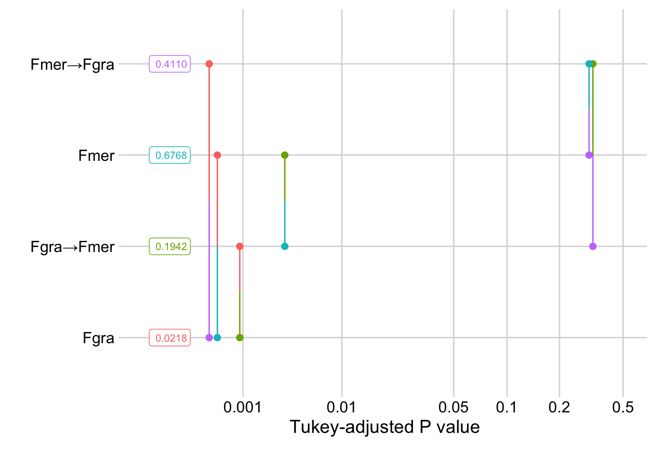

plot estimates

p2 <- medias2$emmeans %>% as.data.frame() %>%
  ggplot(aes(inoculum, response*100, color = inoculum))+
  geom_point(size = 3) +
  geom_errorbar(aes(ymin = lower.CL*100, ymax = upper.CL*100, width = 0))+
   theme_minimal()+
  coord_flip()+
  theme(legend.position="none",
        axis.text.y=element_blank(),
         panel.grid.major.x = element_blank(), 
       #axis.text.x = element_text(angle = 45, hjust = 1),
        #legend.text = element_text(face = "italic", size = 6),
        #strip.text = element_text(face = "italic"),
        plot.margin = margin(0, 0.1, 0.1, 0.1, unit = "cm")
       )+
 labs(y = "GER severity (%)", x ="" )
p2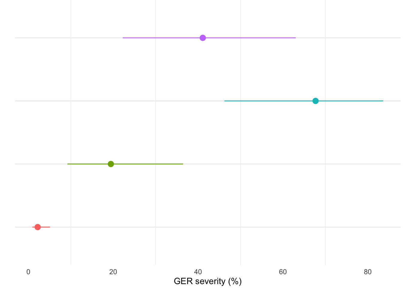

combined plots

library(patchwork)

## 
## Attaching package: 'patchwork'

## The following object is masked from 'package:cowplot':
## 
##     align_plots

## The following object is masked from 'package:MASS':
## 
##     area

p1 + p2 +
 plot_layout(widths = c(2, 1))+
  plot_annotation(tag_levels = 'A')+
  ggsave("figs/Fig-means.png", width = 8, height =3.5)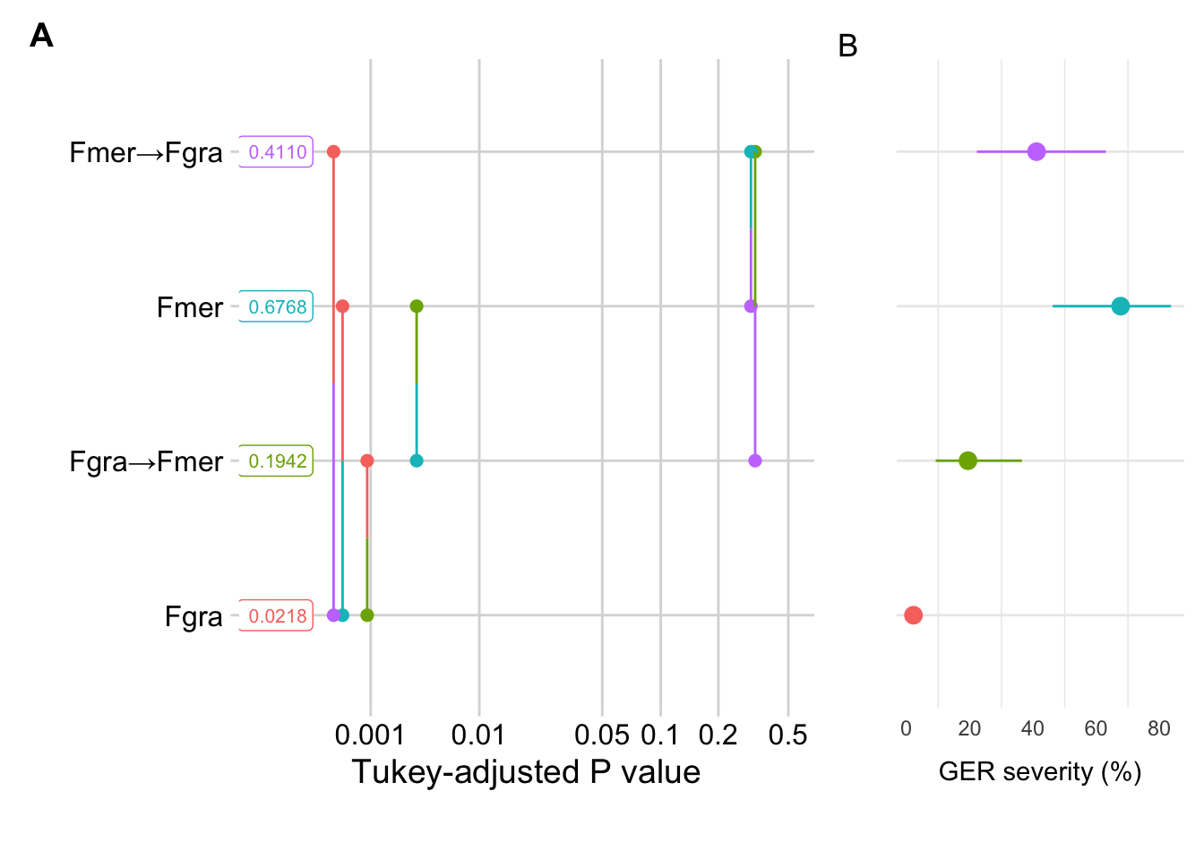

Viçosa trials

Import

dat3 <- read_excel(here("data", "data_field.xlsx"), 1) %>% 
  filter(inoculum != "test" &
         #sev > 0 &
           hybrid != "supremo" &
           trial == "VIC2017"&
           sev != "NA"   )        %>% 
  unite(ambiente, trial, hybrid, sep = ".", remove = F) %>% 
  mutate(sev = as.numeric(sev))

dat3  %>%
  tabyl(inoculum)

dat3 <- dat3 %>% 
  mutate(sev2 = asin(sqrt(sev/100)),
         sev3 = log(sev+0.5),
         sev4 = case_when(sev > 99 ~ 99.9,
                          sev < 1 ~ 0.1,
                          TRUE ~ sev
                          ))

summary(dat3$sev)

##    Min. 1st Qu.  Median    Mean 3rd Qu.    Max. 
##    0.00    4.00    8.00   16.94   22.25  100.00

Visualize

p5 <- dat3 %>% 
    ggplot(aes(x = sev))+
  geom_histogram(binwidth = 5, fill = "steelblue", color = "white")+
  theme_minimal_grid()+
  labs(x = "GER severity (%)", x = "Frequency")

p44 <- dat3 %>% 
    ggplot(aes(x = log(sev)))+
  geom_histogram( fill = "steelblue", color = "white")+
  theme_minimal_grid()+
  labs(x = "log-transformed GER severity", x = "Frequency")

p6 <- dat3 %>% 
  group_by(hybrid, inoculum, block, sev) %>% 
  summarize(sev2 = mean(sev)) %>% 
  ggplot(aes(inoculum, sev2, fill = inoculum, shape = factor(block)))+
  geom_boxplot(outlier.colour = "grey30", alpha = 0.3)+
#geom_jitter(size = 2, width = 0.1,                alpha = 0.2)
  theme_minimal_hgrid()+
  theme(legend.position = "none",
                axis.text.x = element_text(angle = 35, hjust = 1))+  labs(y = "GER severity (%)", x = "Inoculation treatment")

p61 <- dat3 %>% 
  group_by(hybrid, inoculum, block, sev) %>% 
  summarize(sev2 = mean(sev)) %>% 
  ggplot(aes(inoculum, log(sev2), fill = inoculum))+
  geom_boxplot(outlier.colour = NA, alpha = 0.3)+
geom_jitter(size = 2, width = 0.1, 
              shape = 16, alpha = 0.2)+
  theme_minimal_hgrid()+
  theme(legend.position = "none")+
  labs(y = "log-transformed percent severity", x = "Inoculation treatment")

summary(dat3$sev)

##    Min. 1st Qu.  Median    Mean 3rd Qu.    Max. 
##    0.00    4.00    8.00   16.94   22.25  100.00

(p5/p44 | p6) +
 plot_layout(widths = c(1.5,2))+
  plot_annotation(tag_levels = 'A')+
  ggsave("figs/Fig-box2.png", width =10, height =5)

## `stat_bin()` using `bins = 30`. Pick better value with `binwidth`.

## Warning: Removed 7 rows containing non-finite values (stat_bin).

## `stat_bin()` using `bins = 30`. Pick better value with `binwidth`.

## Warning: Removed 7 rows containing non-finite values (stat_bin).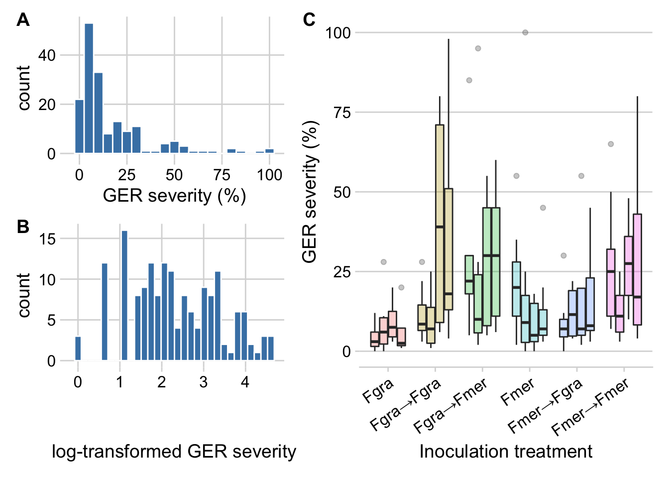

Model

library(glmmTMB)


med2 <- lm(sev3 ~ inoculum, data = dat3 )

AIC(med2)

## [1] 510.5734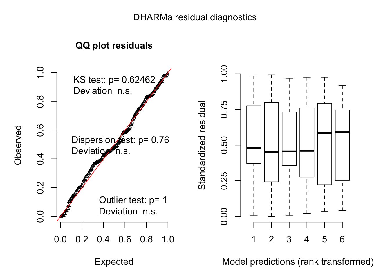

Anova(med2, type = "III")

library(DHARMa)
simres2 <- simulateResiduals(med2)
plot(simres2)

library(emmeans)

medias4 <- emmeans(med2, pairwise ~ inoculum  , type = "response")
CLD(medias4, Lettersfd = LETTERS, alpha = .05)

## Warning: 'CLD' will be deprecated. Its use is discouraged.
## See '? CLD' for an explanation. Use 'pwpp' or 'multcomp::cld' instead.

## Warning in CLD.emm_list(medias4, Lettersfd = LETTERS, alpha = 0.05): `CLD()`
## called with a list of 2 objects. Only the first one was used.

## Warning: 'CLD' will be deprecated. Its use is discouraged.
## See '? CLD' for an explanation. Use 'pwpp' or 'multcomp::cld' instead.

library(cowplot)
p3 <- pwpp(medias4$emmeans, add.space =3, sort = F)+
  theme_minimal_grid()+
  labs(y = "")
p3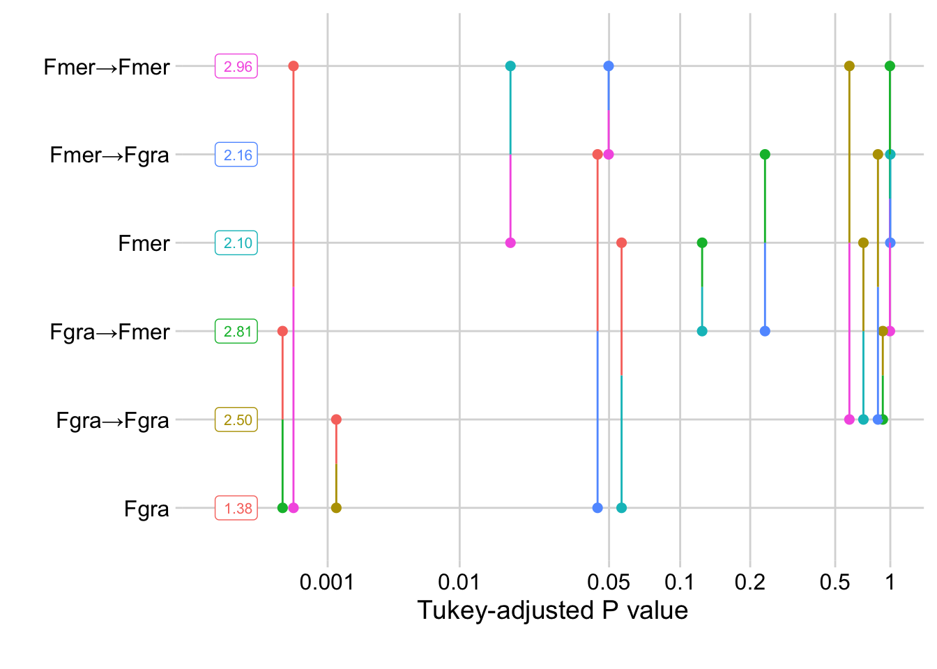

exp(data.frame(medias4$emmeans)$emmean-0.5)

## [1]  2.408033  7.358244 10.062765  4.967081  5.265200 11.687537

p4 <- medias4$emmeans %>% as.data.frame() %>%
  ggplot(aes(inoculum, exp(emmean-0.5), color = inoculum))+
  geom_point(size = 3) +
  geom_errorbar(aes(ymin = exp(lower.CL-0.5), ymax = exp(upper.CL-0.5), width = 0))+
   theme_minimal()+
   coord_flip()+
  theme(legend.position="none",
         axis.text.y=element_blank(),
         panel.grid.major.x = element_blank(), 
       #axis.text.x = element_text(angle = 45, hjust = 1),
        #legend.text = element_text(face = "italic", size = 6),
        #strip.text = element_text(face = "italic"),
        plot.margin = margin(0, 0.1, 0.1, 0.1, unit = "cm")
       )+
 labs(y = "GER severity (%)", x ="" )
p4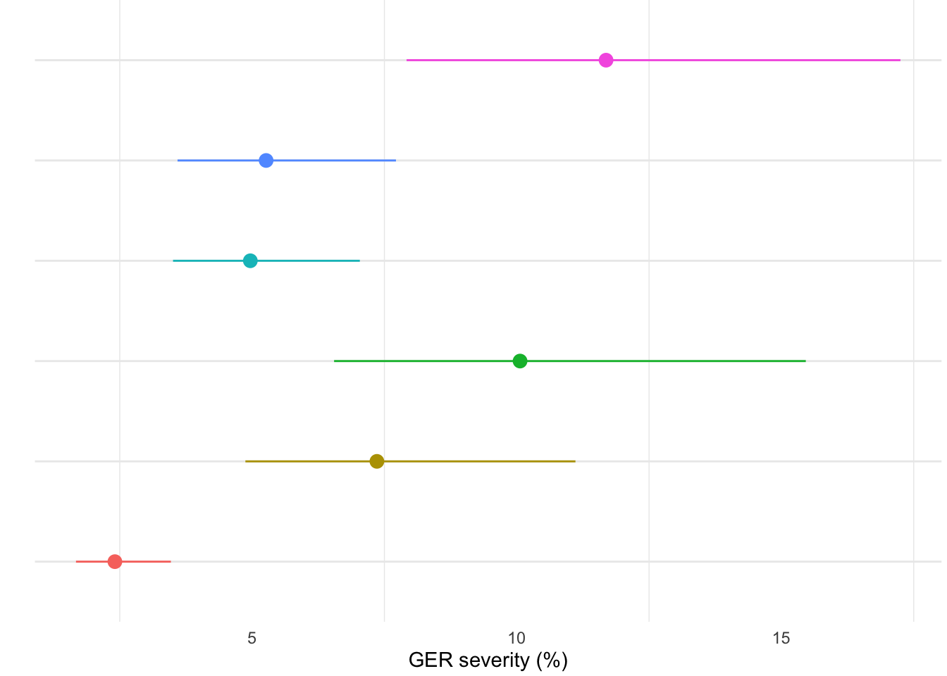

p3 + p4 +
 plot_layout(widths = c(2, 1))+
  plot_annotation(tag_levels = 'A')+
  ggsave("figs/Fig-means2.png", width = 9, height =3.5)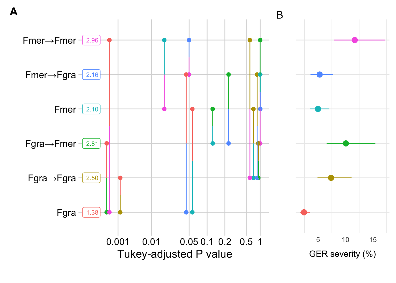

Weather data

library(gsheet)
weather <- gsheet2tbl("https://docs.google.com/spreadsheets/d/1NUG2cdnVNOj1hwyeErQQe1efpFOmUIZVRcA5gxnmT6g/edit#gid=0")

library(tidyverse)
library(cowplot)


  

Ptemp <- weather %>% 
  ggplot(aes(DAI, Tmean, color = Trial, group = Trial))+
  
  geom_errorbar(aes(ymin = Tmin, ymax = Tmax, width =0), size =2, alpha = 0.1)+
  geom_line(size =1)+
  geom_line(aes(DAI, Tmin, color = Trial))+
    geom_line(aes(DAI, Tmax, color = Trial))+
  scale_color_viridis_d(direction =-1)+
  theme_minimal_grid()+
  scale_x_continuous(breaks = seq(-7, 30, 7))+
   scale_y_continuous(breaks = seq(0,45,5), limits = c(0,45))+
  theme(legend.position = "none")+
  facet_wrap(~Trial, nrow = 1)+
    labs(x = "Day Relative to Inoculation", y = "Temperature (C.)")
Ptemp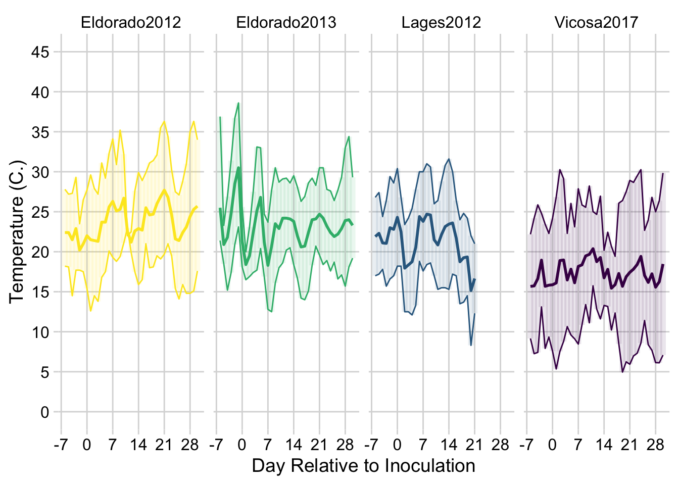

PRH <- weather %>% 
  ggplot(aes(DAI, UR, color = Trial, group = Trial))+
  geom_line(size =1, linetype = 1)+
  scale_color_viridis_d(direction =-1)+
  theme_minimal_grid()+

   scale_x_continuous(breaks = seq(-7, 30, 7))+
     scale_y_continuous(breaks = seq(0,100,5), limits = c(50,100))+
   theme(legend.position = "none")+
  facet_wrap(~ Trial, nrow = 1)+
  labs(x = "Day Relative to Inoculation", y = "Mean relative humidity (%)")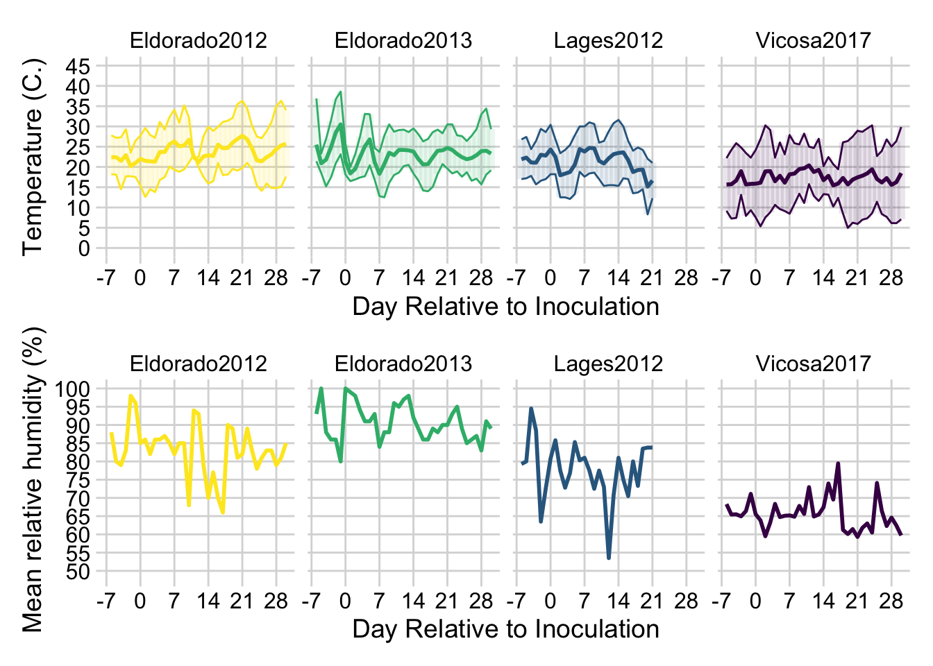

library(patchwork)
Ptemp / PRH +
  ggsave("figs/weather_lines.png", width =9, height =6)

theme_set(theme_minimal_grid(font_size = 10))
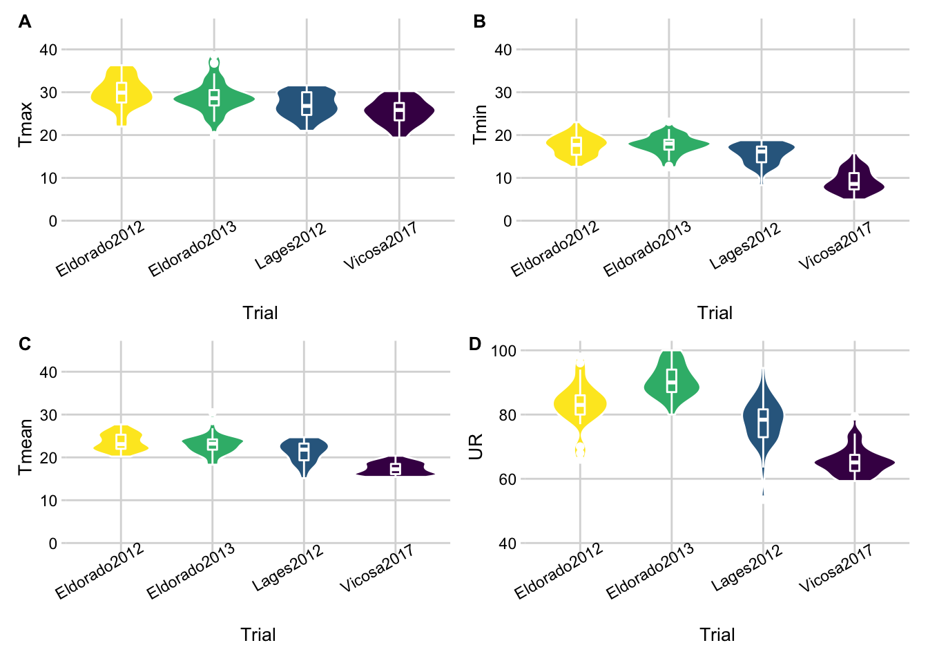
sup_tmean <- weather %>% 
  ggplot(aes(Trial, Tmean, fill = Trial))+
  geom_violin(color = "white")+
  geom_boxplot(width=0.1, color = "white")+
  ylim(0,45)+
   scale_fill_viridis_d(direction =-1)+
  theme(legend.position = "none",
        axis.text.x = element_text(angle = 30, vjust = 1.2, hjust = 0.8))


sup_tmin <- weather %>% 
  ggplot(aes(Trial, Tmin, fill = Trial))+
    geom_violin(color = "white")+
  geom_boxplot(width=0.1, color = "white")+
   ylim(0,45)+
   scale_fill_viridis_d(direction =-1)+
  theme(legend.position = "none",
        axis.text.x = element_text(angle = 30, vjust = 1.2, hjust = 0.8))




sup_tmax <- weather %>% 
  ggplot(aes(Trial, Tmax, fill = Trial))+
  geom_violin(color = "white")+
  geom_boxplot(width=0.1, color = "white")+
   ylim(0,45)+
   scale_fill_viridis_d(direction =-1)+
  theme(legend.position = "none",
        axis.text.x = element_text(angle = 30, vjust = 1.2, hjust = 0.8))


sup_UR <-weather %>% 
  ggplot(aes(Trial, UR, fill = Trial))+
  geom_violin(color = "white")+
  geom_boxplot(width=0.1, color = "white")+
   ylim(40,100)+
   scale_fill_viridis_d(direction =-1)+
  theme(legend.position = "none",
        axis.text.x = element_text(angle = 30, vjust = 1.2, hjust = 0.8))



((sup_tmax | sup_tmin) /
  (sup_tmean | sup_UR))+
  plot_annotation(tag_levels = 'A')+
  ggsave("figs/weather_violin.png", width = 6, height =5)

Code

Load packages

South trials

Visualize

Model fit

Residual

Multiple comparison

pwpp plot

plot estimates

combined plots

Viçosa trials

Import

Visualize

Model

Weather data