figures.utf8.md

Figure 1

Ethiopia Map

library(rnaturalearth)
library(rnaturalearthhires)
library(sf)

## Linking to GEOS 3.7.2, GDAL 2.4.2, PROJ 5.2.0

ETH <- ne_countries(
  country = "Ethiopia",
  returnclass = "sf"
)

region <- sf::st_read("data/ethiopiaregion/Eth_Region_2013.shp")

## Reading layer `Eth_Region_2013' from data source `/Users/emersondelponte/Documents/github/paper-coffee-rust-Ethiopia/data/ethiopiaregion/Eth_Region_2013.shp' using driver `ESRI Shapefile'
## Simple feature collection with 11 features and 6 fields
## geometry type:  MULTIPOLYGON
## dimension:      XY
## bbox:           xmin: -162404.5 ymin: 375657.9 xmax: 1491092 ymax: 1641360
## epsg (SRID):    20137
## proj4string:    +proj=utm +zone=37 +ellps=clrk80 +towgs84=-166,-15,204,0,0,0,0 +units=m +no_defs

zone <- sf::st_read("data/ethiopia-zone/Eth_Zone_2013.shp")

## Reading layer `Eth_Zone_2013' from data source `/Users/emersondelponte/Documents/github/paper-coffee-rust-Ethiopia/data/ethiopia-zone/Eth_Zone_2013.shp' using driver `ESRI Shapefile'
## Simple feature collection with 74 features and 9 fields
## geometry type:  MULTIPOLYGON
## dimension:      XY
## bbox:           xmin: -162404.5 ymin: 375657.9 xmax: 1491092 ymax: 1641360
## epsg (SRID):    20137
## proj4string:    +proj=utm +zone=37 +ellps=clrk80 +towgs84=-166,-15,204,0,0,0,0 +units=m +no_defs

district <- sf::st_read("data/ethiopiaworeda/Eth_Woreda_2013.shp")

## Reading layer `Eth_Woreda_2013' from data source `/Users/emersondelponte/Documents/github/paper-coffee-rust-Ethiopia/data/ethiopiaworeda/Eth_Woreda_2013.shp' using driver `ESRI Shapefile'
## Simple feature collection with 690 features and 12 fields
## geometry type:  MULTIPOLYGON
## dimension:      XY
## bbox:           xmin: -162404.5 ymin: 375657.9 xmax: 1491092 ymax: 1641360
## epsg (SRID):    20137
## proj4string:    +proj=utm +zone=37 +ellps=clrk80 +towgs84=-166,-15,204,0,0,0,0 +units=m +no_defs

ETH_REGIONS <- region %>%
  filter(REGIONNAME %in% c("SNNPR", "Oromia"))

survey$zone <- plyr::revalue(
  survey$zone,
  c(
    "Ilu AbaBora" = "Ilubabor",

    "West Welega" = "West Wellega"
  )
)

## The following `from` values were not present in `x`: West Welega

zone_names <- survey %>%
  select(zone) %>%
  unique()

ETH_ZONE <- zone %>%
  filter(ZONENAME %in% c(
    "Jimma",
    "West Wellega",
    "Sidama",
    "Sheka",
    "Keffa",
    "Bench Maji",
    "Bale",
    "Gedio",
    "Ilubabor"
  ))

district_names <- survey %>%
  select(district) %>%
  unique()

survey$district <- plyr::revalue(survey$district, c(
  "Aira" = "Ayira",
  "Aletawondo" = "Aleta Wendo",
  "Anderecha" = "Anderacha",
  "Debub B" = "Debub Bench",
  "Delo-Menna" = "Mena",
  "Di/Zuria" = "Dila Zuria",
  "Gurafarda" = "Gurafereda",
  "Harena" = "Harena Buluk",
  "Mettu" = "Metu Zuria",
  "Shebe-Sombo" = "Shebe Sambo",
  "Shebedino" = "Shebe Dino",
  "Sheko" = "Sheka",
  "Wonago" = "Wenago",
  "Y/chefe" = "Yirgachefe",
  "Yayo" = "Yayu",
  "Gomma" = "Goma"
))

## The following `from` values were not present in `x`: Aira, Aletawondo, Anderecha, Debub B, Delo-Menna, Di/Zuria, Gurafarda, Harena, Mettu, Shebe-Sombo, Wonago, Y/chefe

district_names <- district_names$district


ETH_DISTRICTS <- district %>%
  filter(WOREDANAME %in% district_names)

survey <- read_csv("data/survey_clean.csv")

Figure 2

Inc-Sev relationship

Figure 3

Incidence vs zone

p_inc_alt_zone <- survey %>%
  ggplot(aes(altitude, logit(inc/100), color = zone, group = zone)) +
  geom_point() +
  geom_smooth(method = lm, se = F) +
  theme_minimal_grid(font_size = 10) +
  theme(legend.position = "none") +
  scale_color_brewer(type = "qual", palette = "Set3")+
    labs(x = "Altitude (m)", y = "Logit Incidence (proportion)")

Severity vs zone

p_sev_alt_zone <- survey %>%
  ggplot(aes(altitude, logit(sev2/100), color = zone, group = zone)) +
  geom_point() +
  geom_smooth(method = lm, se = F) +
  theme_minimal_grid(font_size = 10) +
  theme(legend.position = "none") +
  scale_color_brewer(type = "qual", palette = "Set3")+
    labs(x = "Altitude (m)", y = "Logit Severity (Proportion)")

Plot slopes inc by zone

Effect on incidence

m_alt_inc_zone <- lmer(logit(inc/100 ) ~ altitude * zone + (1 | district), survey, REML = F)
summary(m_alt_inc_zone)

## Linear mixed model fit by maximum likelihood  ['lmerMod']
## Formula: logit(inc/100) ~ altitude * zone + (1 | district)
##    Data: survey
## 
##      AIC      BIC   logLik deviance df.resid 
##    554.9    635.0   -257.5    514.9      385 
## 
## Scaled residuals: 
##     Min      1Q  Median      3Q     Max 
## -3.2089 -0.5685 -0.0957  0.4815  4.6792 
## 
## Random effects:
##  Groups   Name        Variance Std.Dev.
##  district (Intercept) 0.04227  0.2056  
##  Residual             0.18930  0.4351  
## Number of obs: 405, groups:  district, 27
## 
## Fixed effects:
##                             Estimate Std. Error t value
## (Intercept)                0.8510927  0.7852840   1.084
## altitude                  -0.0007735  0.0005239  -1.476
## zoneBench Maji             2.4348759  0.8922217   2.729
## zoneGedio                  2.6106598  1.0325223   2.528
## zoneIlu AbaBora            3.1041604  1.0420872   2.979
## zoneJimma                  2.4720684  1.2604894   1.961
## zoneKeffa                  0.8145031  1.5454408   0.527
## zoneSheka                  3.0386799  1.0261993   2.961
## zoneSidama                 0.8533550  0.9156850   0.932
## zoneWest Wellega           1.5087211  0.9871541   1.528
## altitude:zoneBench Maji   -0.0017946  0.0006112  -2.936
## altitude:zoneGedio        -0.0020325  0.0006646  -3.058
## altitude:zoneIlu AbaBora  -0.0021065  0.0006648  -3.168
## altitude:zoneJimma        -0.0016930  0.0007826  -2.163
## altitude:zoneKeffa        -0.0008470  0.0009272  -0.914
## altitude:zoneSheka        -0.0019962  0.0006671  -2.992
## altitude:zoneSidama       -0.0010900  0.0006004  -1.815
## altitude:zoneWest Wellega -0.0010655  0.0006509  -1.637

## 
## Correlation matrix not shown by default, as p = 18 > 12.
## Use print(x, correlation=TRUE)  or
##     vcov(x)        if you need it

Anova(m_alt_inc_zone, type = "III")

zone_alt_inc <- data.frame(emtrends(m_alt_inc_zone, pairwise ~ zone, var = "altitude" ))

## Warning in (function (..., row.names = NULL, check.rows = FALSE, check.names =
## TRUE, : row names were found from a short variable and have been discarded

p_slopes_inc_alt_zone <- zone_alt_inc %>% 
  ggplot(aes(reorder(emtrends.zone, emtrends.altitude.trend),emtrends.altitude.trend, color = emtrends.zone))+
  geom_point(size =3)+
  coord_flip()+
  theme_minimal_vgrid(font_size = 11)+
  theme(legend.position = "none")+
   scale_color_brewer(type = "qual", palette = "Set3")+
  labs(x = "", y = "Slope estimates")+
  geom_errorbar(aes(ymin = emtrends.lower.CL, ymax = emtrends.upper.CL),
                width =0.2, size =1)

Plots slopes sev by zone

m_alt_sev_zone <- lmer(logit(sev2 ) ~ altitude * zone + (1 | district), data = survey, REML = F)
Anova(m_alt_sev_zone)

zone_alt_sev <- data.frame(emtrends(m_alt_sev_zone, pairwise ~ zone, var = "altitude" ))

## Warning in (function (..., row.names = NULL, check.rows = FALSE, check.names =
## TRUE, : row names were found from a short variable and have been discarded

p_slopes_sev_alt_zone <- zone_alt_sev %>% 
  ggplot(aes(reorder(emtrends.zone, emtrends.altitude.trend),emtrends.altitude.trend, color = emtrends.zone))+
  geom_point(size =3)+
  coord_flip()+
  theme_minimal_vgrid(font_size = 11)+
  theme(legend.position = "none")+
   scale_color_brewer(type = "qual", palette = "Set3")+
  labs(x = "", y = "Slope estimates")+
  geom_errorbar(aes(ymin = emtrends.lower.CL, ymax = emtrends.upper.CL),
                width =0.2, size =1)

Panel of plots

((p_inc_alt_zone  / p_sev_alt_zone ) | (p_slopes_inc_alt_zone / p_slopes_sev_alt_zone)) +
  plot_annotation(tag_levels = "A")

## `geom_smooth()` using formula 'y ~ x'
## `geom_smooth()` using formula 'y ~ x'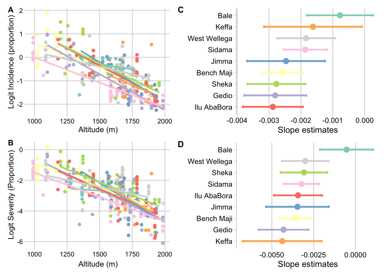

  ggsave("figs/Figure3.png", width = 8, height = 7)

## `geom_smooth()` using formula 'y ~ x'
## `geom_smooth()` using formula 'y ~ x'

Figure 4

Cropping system by zone

survey$cropping_system <- factor(survey$cropping_system, levels = c("Forest", "Semiforest", "Garden", "Plantation"))

csystem <- survey %>% 
  tabyl(zone, cropping_system) %>% 
  gather(cropping_system, name, 2:5)

csystem$cropping_system <- factor(csystem$cropping_system, levels = c("Forest", "Semiforest", "Garden", "Plantation"))

p_cropping <- csystem %>% 
  ggplot(aes(zone, name, fill = cropping_system))+
  geom_col(position = "fill", color = "black", size =0.3)+
  theme(legend.position = "none",
        axis.text.x = element_text(angle = 45, hjust = 1))+
  labs(fill = "",
       x = "",
       y = "Proportion")+
  scale_fill_brewer(palette = "Greens", direction = -1)
p_cropping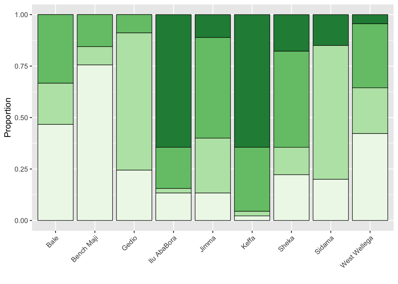

Cropping system by altitude

survey$cropping_system <- factor(survey$cropping_system, levels = c("Forest", "Semiforest", "Garden", "Plantation"))
p_cropping_altitude <- survey %>% 
  dplyr::select(altitude, cropping_system, inc, sev2) %>% 
  ggplot(aes(altitude, logit(sev2), color = cropping_system, group = cropping_system))+
  geom_point(size = 2, shape = 16, alpha = 0.8)+
 # geom_smooth(method = "lm", se = F )+
  theme_minimal_grid(font_size=11)+
  theme(legend.position = "top")+
  labs(color = "",
       x = "Altitude (m)",
       y = "Logit severity")+
  scale_color_brewer(palette = "Greens", direction = -1)
p_cropping_altitude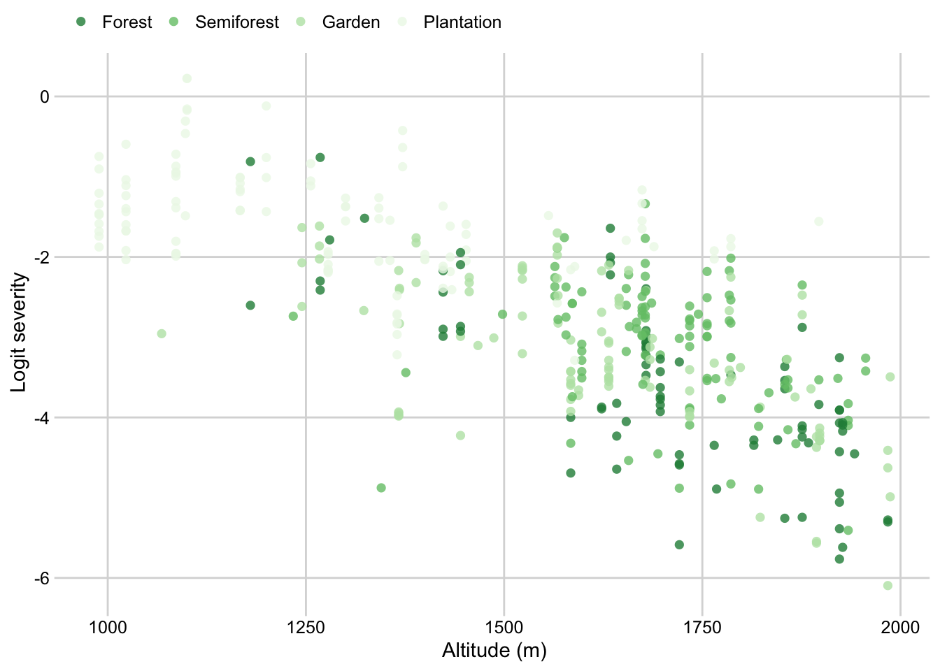

Farm management by zone

farm_man <- survey %>% 
  tabyl(zone, farm_management) %>% 
  gather(farm_management, name, 2:5) 


farm_man$farm_management <- factor(
farm_man$farm_management, levels = c("Intensive", "Moderate", "Minimal", "Unmanaged"))

p_farm <- farm_man %>% 
  ggplot(aes(zone, name, fill = farm_management))+
  geom_col(position = "fill", color = "black", size =0.3)+
  theme(legend.position = "none",
        axis.text.x = element_text(angle = 45, hjust = 1))+
  labs(fill = "",
       x = "",
       y = "Proportion")+
  scale_fill_brewer(palette = "Blues", direction = -1)

Farm management by altitude

survey$farm_management <- factor(
survey$farm_management, levels = c("Intensive", "Moderate", "Minimal", "Unmanaged"))
p_farm_man_altitude <- survey %>% 
  dplyr::select(altitude, farm_management, inc, sev2) %>% 
  ggplot(aes(altitude, logit(sev2), color = farm_management, group = farm_management))+
  geom_point(size = 2, shape = 16, alpha = 0.8)+
 # geom_smooth(method = "lm", se = F )+
  theme_minimal_grid(font_size=11)+
  theme(legend.position = "top")+
  labs(color = "",
       x = "Altitude (m)",
       y = "Logit severity")+
scale_color_brewer(palette = "Blues", direction = -1)
p_farm_man_altitude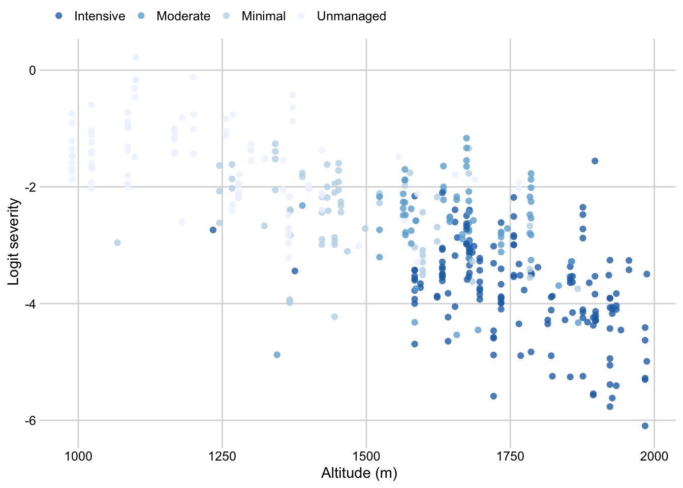

Shade by zone

library(janitor)
survey_shade <- survey %>% 
  tabyl(zone, shade) %>% 
  gather(shade, name, 2:4) 


survey_shade$shade <- factor(
survey_shade$shade, levels = c("Full shade", "Mid shade", "Sun"))

p_shade <- survey_shade %>% 
  ggplot(aes(zone, name, fill = shade))+
  geom_col(position = "fill", color = "black", size =0.3)+
  theme(legend.position = "none",
        axis.text.x = element_text(angle = 45, hjust = 1))+
  labs(fill = "",
       x = "",
       y = "Proportion")+
  scale_fill_brewer(palette = "OrRd", direction = 1)
p_shade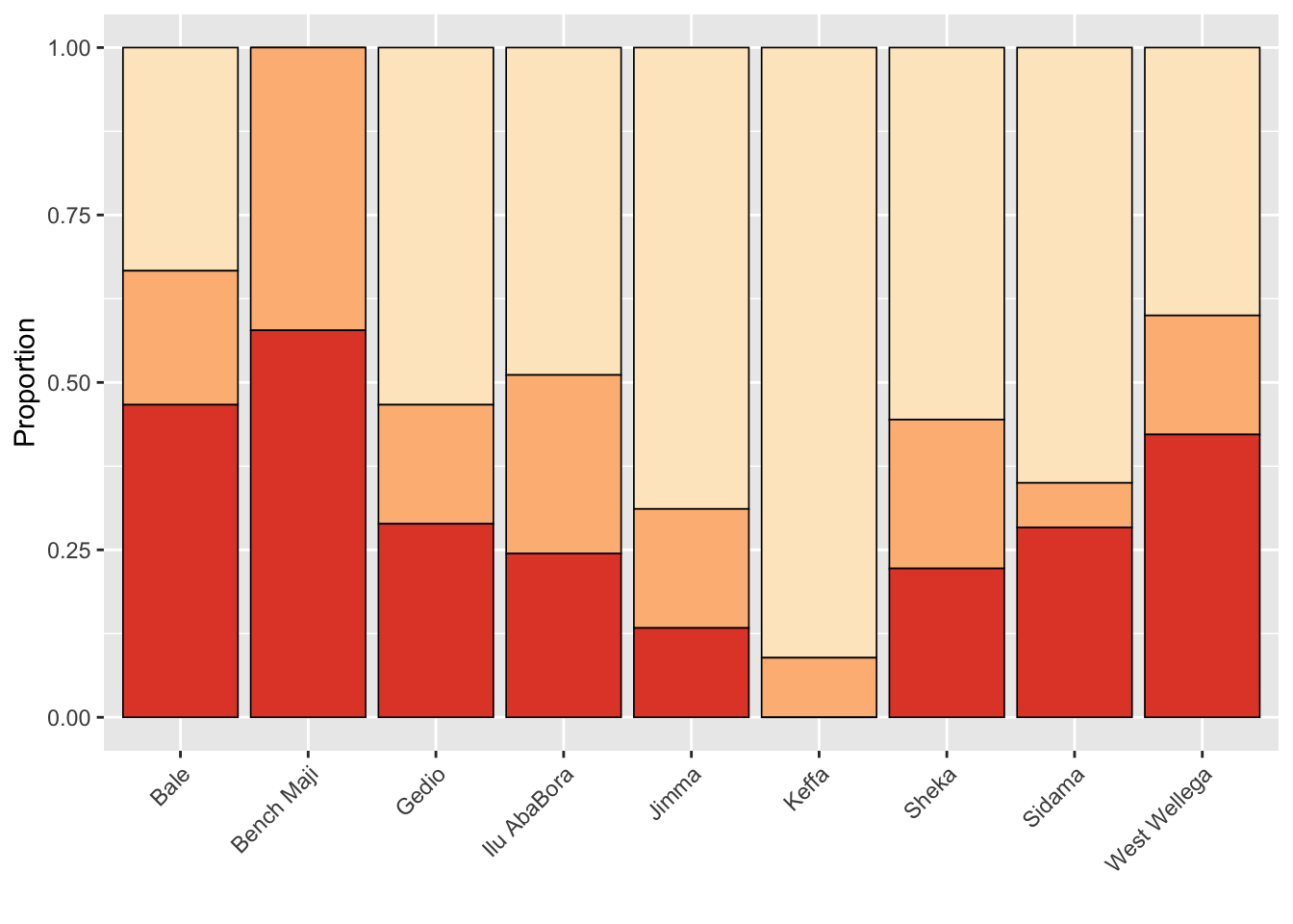

Shade by altitude

survey$shade <- factor(
survey$shade, levels = c("Full shade", "Mid shade", "Sun"))

p_shade_altitude <- survey %>% 
  dplyr::select(altitude, shade, inc, sev2) %>% 
  ggplot(aes(altitude, logit(sev2), color = shade, group = shade))+
  geom_point(size = 2, shape = 16, alpha = 0.8)+
 # geom_smooth(method = "lm", se = F )+
  theme_minimal_grid(font_size=11)+
  theme(legend.position = "top")+
  labs(color = "",
       x = "Altitude (m)",
       y = "Logit severity")+
  scale_color_brewer(palette = "OrRd", direction = 1)
p_shade_altitude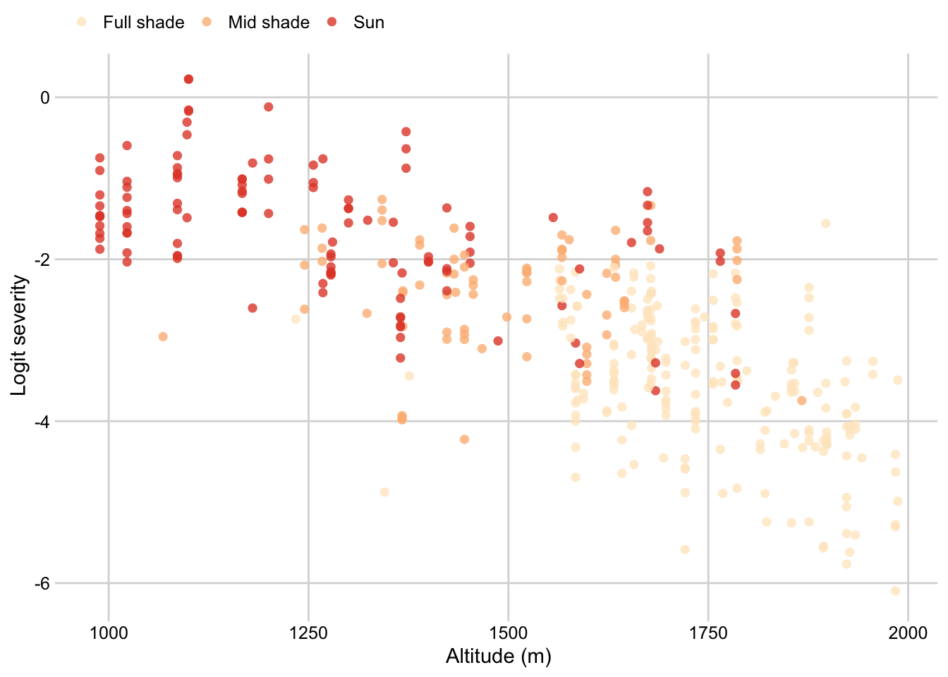

Cultivar by zone

survey_cult <-survey %>% 
  tabyl(zone, cultivar) %>% 
  gather(cultivar, name, 2:4) 
  

survey_cult$cultivar <- factor(

survey_cult$cultivar, levels = c("Improved", "Mixture", "Local", "Unmanaged"))

p_cult <- survey_cult %>% 
  ggplot(aes(zone, name, fill = cultivar))+
  geom_col(position = "fill", color = "black", size =0.3)+
  theme(legend.position = "none",
        axis.text.x = element_text(angle = 45, hjust = 1))+
  labs(fill = "",
       x = "",
       y = "Proportion")+
  scale_fill_brewer(palette = "PuRd", direction = -1)
p_cult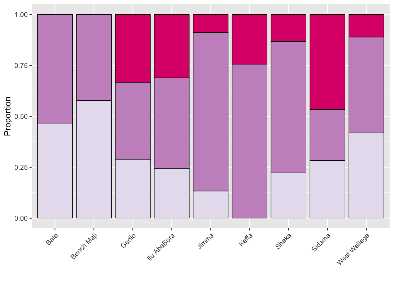

Cultivar by altitude

survey$cultivar <- factor(

survey$cultivar, levels = c("Improved", "Mixture", "Local", "Unmanaged"))
p_cult_altitude <- survey %>% 
  dplyr::select(altitude, cultivar, inc, sev2) %>% 
  ggplot(aes(altitude, logit(sev2), color = cultivar, group = cultivar))+
  geom_point(size = 2, shape = 16, alpha = 0.8)+
 # geom_smooth(method = "lm", se = F )+
  theme_minimal_grid(font_size=11)+
  theme(legend.position = "top")+
  labs(color = "",
       x = "Altitude (m)",
       y = "Logit severity")+
  scale_color_brewer(palette = "PuRd", direction = -1)
p_cult_altitude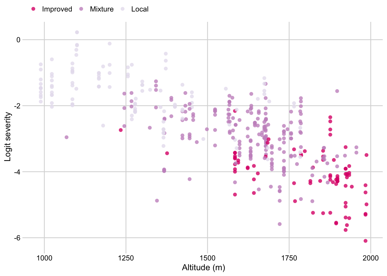

Compose figure

library(patchwork)

 ((p_cropping_altitude / p_cult_altitude / p_farm_man_altitude / p_shade_altitude) |
  ((p_cropping / p_cult /p_farm / p_shade ) ))+ 
      plot_annotation(tag_levels = 'A')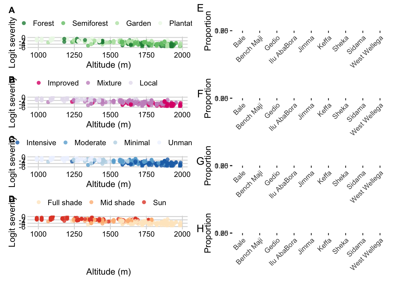

ggsave("figs/Figure4.png", width =8, height =10)

(p_cropping_altitude / p_cult_altitude / p_farm_man_altitude / p_shade_altitude))+

Figure 5

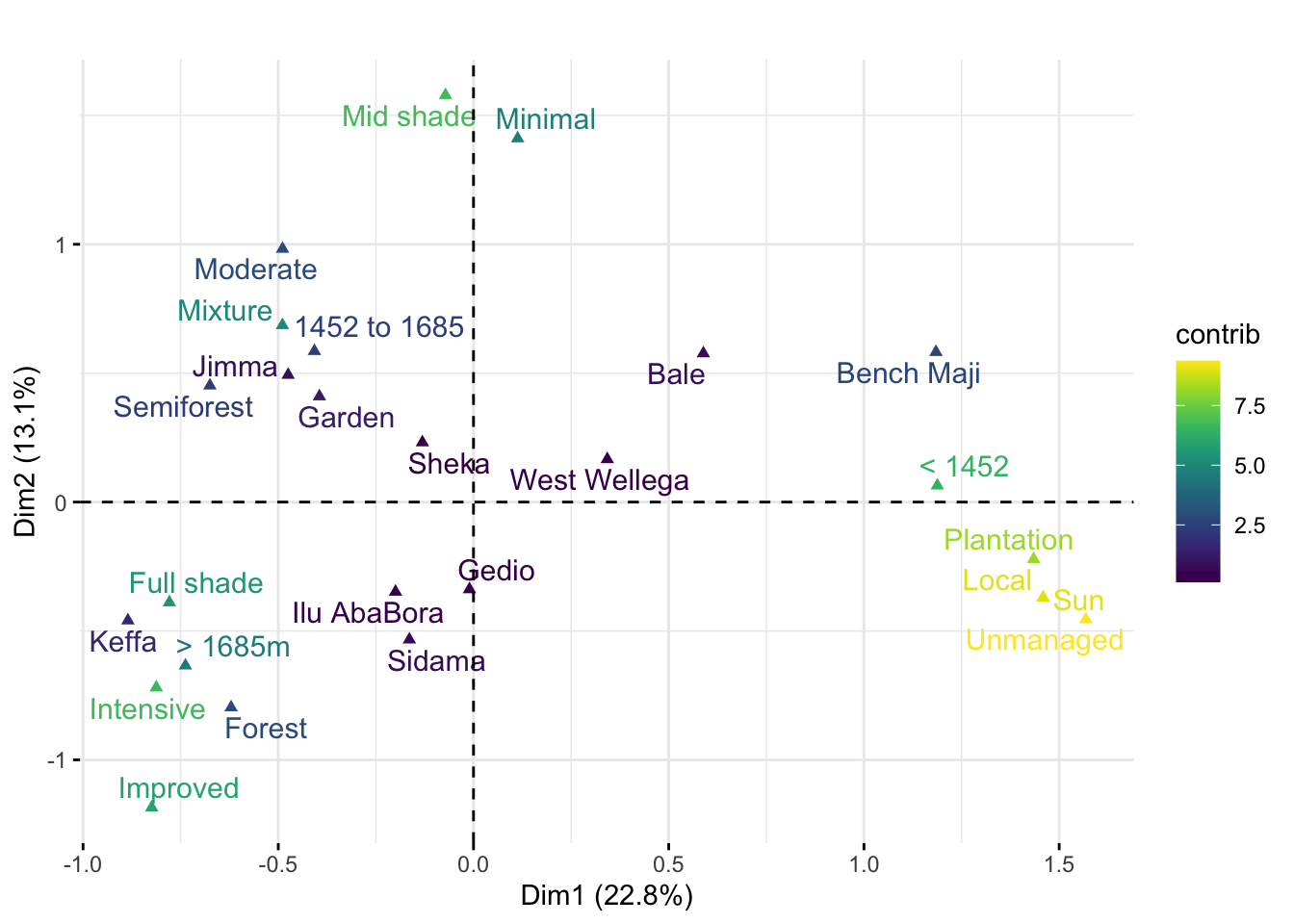
MCA plot

library(FactoMineR)
library(factoextra)

## Welcome! Related Books: `Practical Guide To Cluster Analysis in R` at https://goo.gl/13EFCZ

survey_mca <- survey %>% 
 mutate(altitude2 = case_when(
    altitude < 1452 ~ "< 1452",
    altitude < 1685 ~ "1452 to 1685",
    TRUE ~ "> 1685m"
  )) 
 
attach(survey_mca)

## The following objects are masked _by_ .GlobalEnv:
## 
##     district, region, zone

data_mca <- survey_mca %>% dplyr::select(altitude2, zone, cultivar, shade, cropping_system, farm_management)

head(data_mca)

cats <- apply(data_mca, 2, function(x) nlevels(as.factor(x))) # enumera as categorias
cats

##       altitude2            zone        cultivar           shade cropping_system 
##               3               9               3               3               4 
## farm_management 
##               4

res.mca <- MCA(data_mca, graph = FALSE)

p <- fviz_mca_var(res.mca,
  label = "var", repel = T,
  col.var = "contrib",
  # Avoid text overlapping (slow if many point)
  ggtheme = theme_minimal()
)
p + scale_color_viridis() +
  labs (title = "", fill = "Contribution")+
  ggsave("figs/Figure5.png", width =7, height =5)

Figures

Figure 1

Ethiopia Map

Figure 2

Inc-Sev relationship

Figure 3

Incidence vs zone

Severity vs zone

Plot slopes inc by zone

Effect on incidence

Plots slopes sev by zone

Panel of plots

Figure 4

Cropping system by zone

Cropping system by altitude

Farm management by zone

Farm management by altitude

Shade by zone

Shade by altitude

Cultivar by zone

Cultivar by altitude

Compose figure

Figure 5

MCA plot