Analysis code

Load libraries

library(plyr) # for data transformation
library(tidyverse) # tidy tools
library(readxl) # import from excel
library(epiR) # ccc analysis
library(ggthemes) # ggplot themes
library(irr) # icc analysis
library(rel) # agreement analysis
theme_set(theme_light()) # the theme globally

Data preparation

Import

Import the raw data stored in a xlsx file using the read_excel function of the readxl package.

dat_cls <- read_excel("data/data-sad-cls.xlsx", 1)

Reshape

We need to reshape the data from the wide (rating systems in different columns) to the long format where each row is an observation, or a leaf in our case. There are three response variables of interest:

actual severity
estimate of severity using the different systems
error of the estimates (estimate - actual).

The error variable is created below using the mutate function.

dat_sad <- dat_cls %>%
  gather(assessment, estimate, 4:8) %>%
  mutate(error = estimate - actual)

dat_sad

Transform

Since we are using ordinal scales like Horsfall-Barrat (HB) and a 10% linear interval scale (LIN), we need convert the actual and estimates of severity to the corresponding ordinal value. By doing this we can inspect errors associated with the assignment of a wrong score. The new variables will be named: actual_HB, actual_LIN, estimate_HB and estimate_LI. Thecase_when` function is very handy for this task.

dat_sad <- dat_sad %>%
  mutate(actual_HB = case_when(
    actual < 3 ~ 1,
    actual < 6 ~ 2,
    actual < 12 ~ 3,
    actual < 25 ~ 4,
    actual < 50 ~ 5,
    actual < 75 ~ 6,
    actual < 88 ~ 7,
    actual < 94 ~ 8,
    actual < 97 ~ 9,
    actual < 100 ~ 10
  ))

dat_sad <- dat_sad %>%
  mutate(actual_LIN = case_when(
    actual < 10 ~ 1,
    actual < 20 ~ 2,
    actual < 30 ~ 3,
    actual < 40 ~ 4,
    actual < 50 ~ 5,
    actual < 60 ~ 6,
    actual < 70 ~ 7,
    actual < 80 ~ 8,
    actual < 90 ~ 9,
    actual < 100 ~ 10
  ))

dat_sad <- dat_sad %>%
  mutate(estimate_HB = case_when(
    estimate < 3 ~ 1,
    estimate < 6 ~ 2,
    estimate < 12 ~ 3,
    estimate < 25 ~ 4,
    estimate < 50 ~ 5,
    estimate < 75 ~ 6,
    estimate < 88 ~ 7,
    estimate < 94 ~ 8,
    estimate < 97 ~ 9,
    estimate < 100 ~ 10
  ))

dat_sad <- dat_sad %>%
  mutate(estimate_LIN = case_when(
    estimate < 10 ~ 1,
    estimate < 20 ~ 2,
    estimate < 30 ~ 3,
    estimate < 40 ~ 4,
    estimate < 50 ~ 5,
    estimate < 60 ~ 6,
    estimate < 70 ~ 7,
    estimate < 80 ~ 8,
    estimate < 90 ~ 9,
    estimate < 100 ~ 10
  ))

Visualize

We will make use of a range of techniques to visualize the data from all assessment rounds. Firstly, let’s explore data for the unaided estimates to check the variability in the innate ability of the raters and types of errors.

Unaided

In the unaided assessment the raters provided direct estimates of percent severity without any aid, but only based on their perception of the percent diseased leaf area. Let’s inspect the distribution of the values for the unaided estimates of severity across the range of percent scale for all raters combined. Compare them with the actual severity depicted as rugs at the x scale.

actual <- dat_cls %>%
  filter(rater == 1) %>%
  select(actual)

dat_sad %>%
  filter(assessment == "UN") %>%
  select(rater, actual, estimate) %>%
  ggplot(aes(estimate)) +
  scale_x_continuous(breaks = seq(0, 100, 5)) +
  #geom_vline(aes(xintercept = actual), linetype = 2, color = "gray80", size = 0.5) +
  theme_light()+
  geom_rug(aes(actual))+
  geom_histogram(bins = 100, color = "white", fill = "gray50") +

  labs(x = "Nearest percent unaided estimate", y = "Frequency") +
  ggsave("figs/figs1.png", width = 7, height = 3, dpi = 300)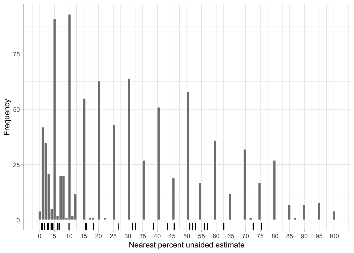

It is quite apparent that raters tended to round the estimates around a “knot” spaced at 10 percent points. Let’s calculate the frequency of the ten most assigned values. The janitor package is useful to get the percent as well as the cumulative percent for each value, ordered from high to low.

library(janitor)
dat_sad %>%
  filter(assessment == "UN") %>%
  tabyl(estimate) %>%
  arrange(-n) %>%
  mutate(cum_percent = cumsum(percent))

Based on the above, ten values accounted for 66% of the assigned values. The top five were 10%, 5%, 30%, 20% and 50%. Apparently, raters intuitively used a mental linear scale to assign severity.

Errors

The plot below shows the relationship between the errors of the estimates, in percent points, and the actual severity values.

fig4a <- dat_sad %>%
  filter(assessment == "UN") %>%
  ggplot(aes(actual, error)) +
   theme_light()+
  theme(legend.position = "none") +
  geom_hline(yintercept = 0) +
  coord_fixed() +
  geom_point(alpha = 0.5, size = 2.5, shape = 16) +
  labs(
    x = "Actual severity (%)",
    y = "Error of estimates (percentage point)"
  ) 

fig4a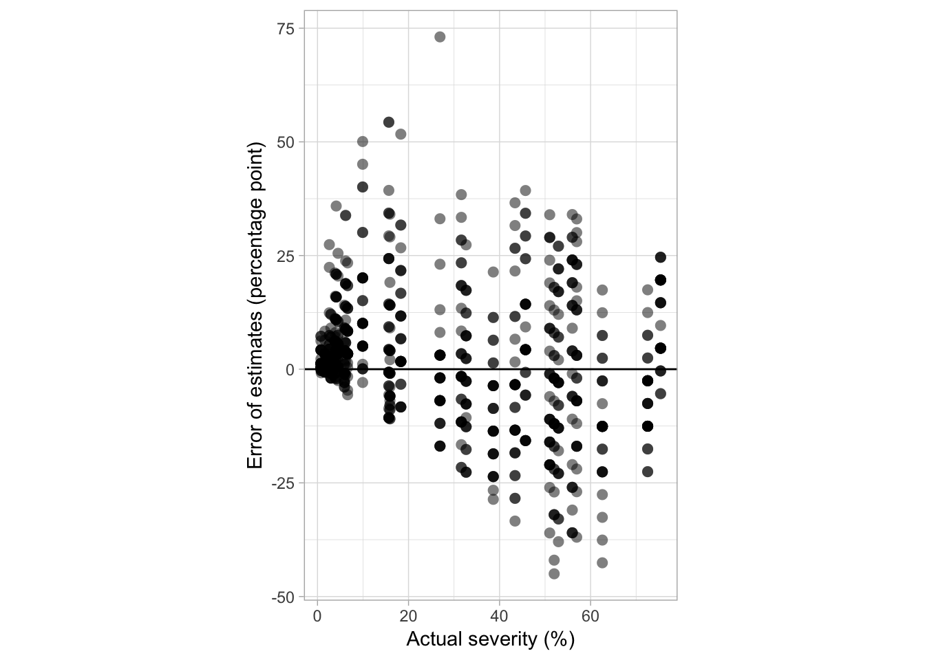

Aided

Let’s now check the distribution of the aided estimates for each of the aid systems.

knots_aid <- dat_sad %>%
  filter(assessment != "UN") %>%
  ggplot(aes(estimate)) +
  #geom_vline(aes(xintercept = actual), linetype = 1, color = "gray", size = 0.5) +
  geom_rug(aes(actual))+
  geom_histogram(bins = 100, color = "white", fill = "gray50") +
   theme_light()+
   facet_wrap(~ assessment, ncol = 1) +
 labs(x = "Aided Estimate", y = "Frequency")+
  scale_x_continuous(breaks = seq(0, 100, 5), limits = c(0, 100)) +
  ggsave("figs/figs2.png", width = 5, height = 6, dpi = 600)

When using the H-B scale, all mid-point severity values showed higher frequency for the 4.5% scores. This was expected given the higher frequency of actual values at the lower end of the percent scale.

For the two two-stage assessment, it seems the knots were still preferred by the raters for the range of values within the category. Let’s get the frequency of the ten most assigned values after selecting a score following the log for the linear interval.

First, the log interval scale. The tabyl function of the janitor package provides a nice output.

library(janitor)
dat_sad %>%
  filter(assessment == "HB2") %>%
  tabyl(estimate) %>%
  arrange(-n) %>%
  mutate(cum_percent = cumsum(percent)) %>%
  head(10)

In fact, more than fifty percent of the severity values were assigned to only ten values, which are mostly in the middle of the interval.

Now frequency of estimates using the linear scale.

library(janitor)
dat_sad %>%
  filter(assessment == "LIN2") %>%
  tabyl(estimate) %>%
  arrange(-n) %>%
  mutate(cum_percent = cumsum(percent)) %>%
  head(10)

Again, raters tend to round their estimates to a knot or the score of the linear interval scale. Seventy percent of the estimates were comprised of 10 values, with 50%, 5%, 10%, 2%, 20% and 40% contributing to 50% of the estimates. Of those, only 2% and 5% are not cut-off values.

dat_sad %>%
  filter(assessment != "UN") %>%
  ggplot(aes(actual, error)) +
  coord_fixed() +
  xlim(0, 90) +
  geom_point(alpha = 0.3, size = 2) +
  geom_smooth(color = "orange", size = 1.5, linetype = 1, se = F) +
  geom_hline(yintercept = 0) +
   theme_light()+
  theme(legend.position = "none") +
  facet_wrap(~ assessment, ncol = 4) +
  labs(y = "Error (percentage point)", x = "Actual severity (%)") +
  ggsave("figs/fig6.png", width = 8, dpi = 600)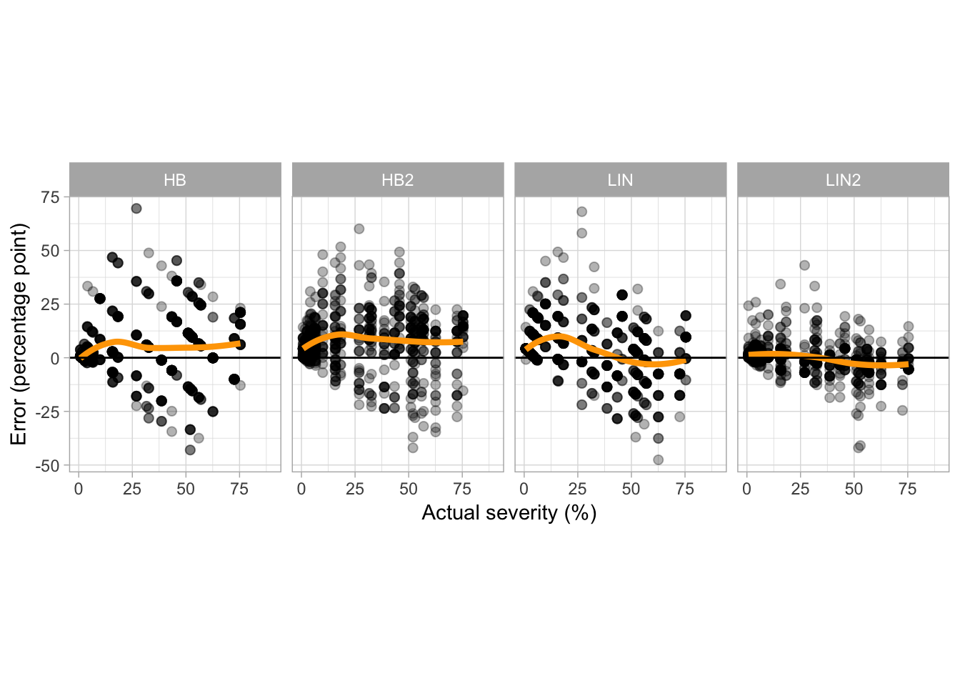

For most cases, overestimation occurred at values lower than 30% actual severity, especially for the aided estimates using the LIN scale and UN estimates. However, when using the HB scale the overestimation was more consistent across the entire severity range.

Ordinal data

Now let’s see the errors of estimates when using ordinal scales. First, we will summarize the frequency of the correct assignment. Then, we build a contingency table for the estimated versus actual scores and count the proportion of data on the correct class and those nearby.

hb_table <- dat_sad %>%
  filter(assessment == "HB") %>%
  tabyl(actual_HB, estimate_HB) %>%
  adorn_percentages("row") %>%
  round(2)
hb_table

We can now produce a heat map of the frequencies for better visualization.

p_hb_table <- hb_table %>%
  gather(HB, value, 2:11) %>%
  mutate(HB = as.numeric(HB)) %>%
  ggplot(aes(actual_HB, HB, fill = value)) +
  geom_tile() +
  geom_text(aes(label = value), color = "white", size = 3) +

  scale_y_continuous(breaks = seq(1, 9, 1)) +
  scale_x_continuous(breaks = seq(1, 9, 1)) +
  scale_fill_gradient(low = "white", high = "black") +
  theme_few()+
  theme(legend.position = "none") +
  labs(x = "Actual HB class", fill = "Proportion", y = "Estimated HB class")
p_hb_table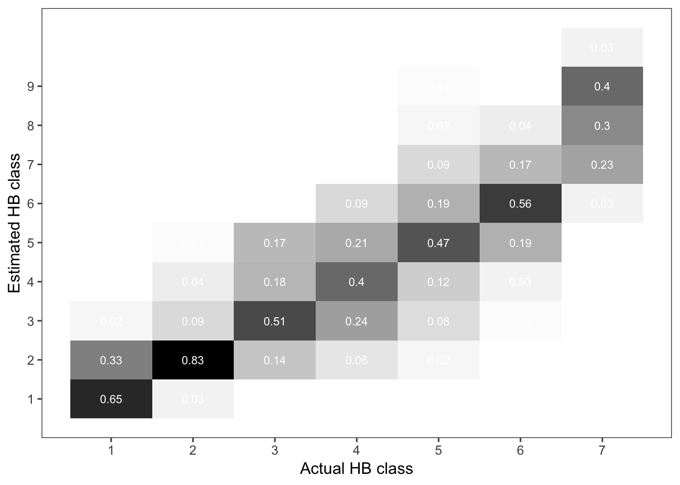

Now, we repeat the procedure for the LIN scale.

lin_table <- dat_sad %>%
  filter(assessment == "LIN") %>%
  tabyl(actual_LIN, estimate_LIN) %>%
  adorn_percentages("row") %>%
  round(2)
lin_table

and another heat map.

p_lin_table <- lin_table %>%
  gather(LIN, value, 2:11) %>%
  mutate(LIN = as.numeric(LIN)) %>%
  ggplot(aes(actual_LIN, LIN, fill = value)) +
  geom_tile() +
  geom_text(aes(label = value), color = "white", size = 3) +
  scale_y_continuous(breaks = seq(1, 9, 1)) +
  scale_x_continuous(breaks = seq(1, 9, 1)) +
  scale_fill_gradient(low = "white", high = "black") +
  theme_few()+
  labs(x = "Actual LIN class", fill = "Proportion", y = "Estimated LIN class")

p_lin_table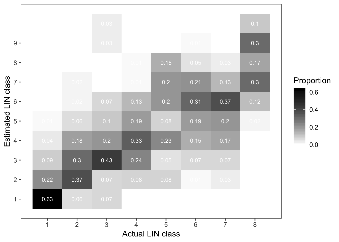

Here we will make a combo plot with the two graphs using the plot_grid function of the cowplot package.

library(cowplot)
theme_set(theme_light())
p1 <- plot_grid(p_hb_table, p_lin_table, align = "hv", ncol = 2, rel_widths = c(1, 1.35), labels = "AUTO")
ggsave("figs/fig5.png", p1, width = 9)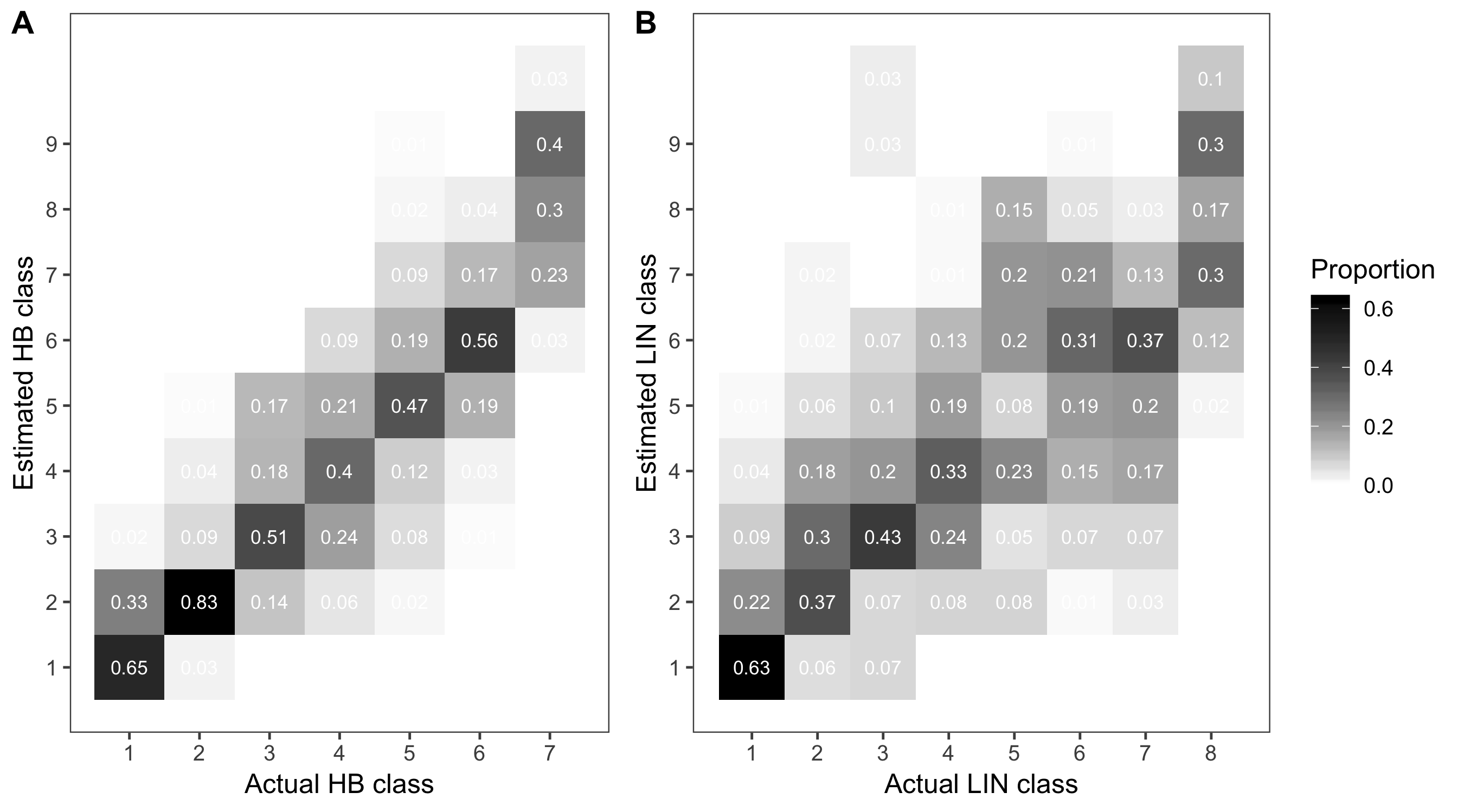

Agreement stats

Here will compute a simple percentage agreement and a weighted Kappa statistics (for ordered categories with quadratic weights) between the estimated and actual ordinal categories.

HB

Percent agreement

HB <- dat_sad %>%
  filter(assessment == "HB") %>%
  select(actual_HB, estimate_HB)
library(irr)
agree(HB, tolerance = 0)

##  Percentage agreement (Tolerance=0)
## 
##  Subjects = 900 
##    Raters = 2 
##   %-agree = 57

Weighted Kappa statistics is calculated using the rel package.

# weighted Kappa for ordered categories with quadratic weights
library(rel)
ckap(weight = "quadratic", data = HB)

## Call:
## ckap(data = HB, weight = "quadratic")
## 
##        Estimate    StdErr   LowerCB UpperCB
## Const 0.8916350 0.0069943 0.8779079  0.9054
## 
## Maximum kappa = -0.37
## Kappa/maximum kappa = -2.38
## Confidence level = 95%
## Observations = 2
## Sample size = 900

kappa2(HB, weight = "squared")

##  Cohen's Kappa for 2 Raters (Weights: squared)
## 
##  Subjects = 900 
##    Raters = 2 
##     Kappa = 0.889 
## 
##         z = 26.8 
##   p-value = 0

LIN

Percent agreement

LIN <- dat_sad %>%
  filter(assessment == "LIN") %>%
  select(actual_HB, estimate_HB)
# % agreement
agree(LIN, tolerance = 2)

##  Percentage agreement (Tolerance=2)
## 
##  Subjects = 900 
##    Raters = 2 
##   %-agree = 97

Weighted Kappa

ckap(weight = "quadratic", data = LIN)

## Call:
## ckap(data = LIN, weight = "quadratic")
## 
##       Estimate   StdErr  LowerCB UpperCB
## Const 0.826541 0.010532 0.805871  0.8472
## 
## Maximum kappa = -1.37
## Kappa/maximum kappa = -0.6
## Confidence level = 95%
## Observations = 2
## Sample size = 900

Two-stage estimation

Now we want to see the distribution of the severity values (second step) assigned within each score chosen in the first step. The goal is to check whether there was a tendency to assign specific values.

HB

HB_hist <- dat_sad %>%
  filter(assessment == "HB2") %>%
  select(estimate, estimate_HB) %>%
  gather(class, value, 2) %>%
  ggplot(aes(estimate)) +
   theme_light()+
  geom_histogram(bins = 100, color = "white") +
  labs(x = "Percent estimate after H-B scale", y = "Frequency") +
  scale_x_continuous(breaks = seq(0, 100, 5), limits = c(0, 100)) +
  theme(legend.position = "none")

LIN

LIN_hist <- dat_sad %>%
  filter(assessment == "LIN2") %>%
  select(estimate, estimate_LIN) %>%
  gather(class, value, 2) %>%
  ggplot(aes(estimate)) +
  geom_histogram(bins = 100, color = "white") +

  scale_x_continuous(breaks = seq(0, 100, 5), limits = c(0, 100)) +
   theme_light()+
  theme(legend.position = "none") +
  labs(x = "Percent estimate after 10% Linear scale", y = "Frequency")

The combo plot for the supplemental section of the manuscript.

library(cowplot)
theme_set(theme_light())
p_hist <- plot_grid(HB_hist, LIN_hist, align = "hv", ncol = 1, rel_widths = c(1, 1), labels = "AUTO")
ggsave("figs/fig4.png", p_hist, width = 6, height = 5)
p_hist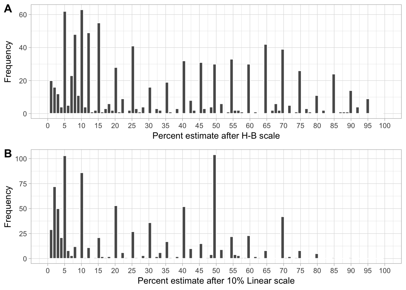

Concordance analysis

Lin’s statistics

The Lin’s concordance correlation coefficient provides a measure of overall accuracy which takes into account bias correction (closeness to the actual value) and precision (variability in the estimates). Bias correction is calculated from two bias measures: constant bias (location-shift) and systematic bias (scale-shift). The precision is the Pearson’s correlation coefficient. The concordance correlation (CCC) is the product of bias correction and precision.

We will use the epi.ccc function of the epiR package to obtain the CCC statistics for each of the five assessments.

Unaided

dat_sad_UN <- dat_sad %>%
  group_by(rater) %>%
  filter(assessment == "UN")
ccc_UN <- by(dat_sad_UN, dat_sad_UN$rater, function(dat_sad_UN)
  epi.ccc(dat_sad_UN$actual, dat_sad_UN$estimate, ci = "z-transform", conf.level = 0.95))

LIN

library(irr)
dat_sad_estimate_LIN <- dat_sad %>%
  group_by(rater) %>%
  filter(assessment == "LIN")
ccc_estimate_LIN <- by(dat_sad_estimate_LIN, dat_sad_estimate_LIN$rater, function(dat_sad_estimate_LIN)
  epi.ccc(dat_sad_estimate_LIN$actual, dat_sad_estimate_LIN$estimate, ci = "z-transform", conf.level = 0.95))

LIN2

dat_sad_estimate_LIN2 <- dat_sad %>%
  group_by(rater) %>%
  filter(assessment == "LIN2")
ccc_estimate_LIN2 <- by(dat_sad_estimate_LIN2, dat_sad_estimate_LIN2$rater, function(dat_sad_estimate_LIN2)
  epi.ccc(dat_sad_estimate_LIN2$actual, dat_sad_estimate_LIN2$estimate, ci = "z-transform", conf.level = 0.95))

LOG

dat_sad_estimate_HB <- dat_sad %>%
  group_by(rater) %>%
  filter(assessment == "HB")
ccc_estimate_HB <- by(dat_sad_estimate_HB, dat_sad_estimate_HB$rater, function(dat_sad_estimate_HB)
  epi.ccc(dat_sad_estimate_HB$actual, dat_sad_estimate_HB$estimate, ci = "z-transform", conf.level = 0.95))

LOG2

dat_sad_estimate_HB2 <- dat_sad %>%
  group_by(rater) %>%
  filter(assessment == "HB2")
ccc_estimate_HB2 <- by(dat_sad_estimate_HB2, dat_sad_estimate_HB2$rater, function(dat_sad_estimate_HB2)
  epi.ccc(dat_sad_estimate_HB2$actual, dat_sad_estimate_HB2$estimate, ci = "z-transform", conf.level = 0.95))

Combined all data

We created the five tibbles and now we combine everything in a same tibble. The rbind function of the base R does the job.

ccc_all <- rbind(
  ccc_UN_df,
  ccc_estimate_LIN2_df,
  ccc_estimate_LIN_df,
  ccc_estimate_HB2_df,
  ccc_estimate_HB_df
)
ccc_all

Note that the data in ccc_all are in the wide format, where each statistics is shown in a different column. We will change it to the long format using the gather function.

ccc <- ccc_all %>%
  gather(stat, coef, 2:6)

Baseline accuracy

We will produce a plot to depict the relationship between the bias coefficient and the Pearson’s coefficient for the unaided estimates. We want to depict the differences in accuracy among the raters while visualizing the three coefficients, including the concordance correlation.

We will filter the UN estimates and not use the two components of bias.

UN_CCC <- ccc %>%
  filter(
    method == "UN",
    stat != "l.shift",
    stat != "s.shift"
  ) %>%
  select(rater, stat, coef) %>%
  arrange(desc(coef))

UN_CCC2 <- UN_CCC %>%
  spread(stat, coef)

Now a linear model for the relationship between Cb and r. We extract the correlation coefficient of the relationship.

linear_model <- function(df) {
  lm(
    Cb ~ r,
    data = UN_CCC2
  )
}
modelo <- UN_CCC2 %>%
  linear_model()
sqrt(summary(modelo)$r.squared)

## [1] 0.9564612

Now the plot for the manuscript.

fig4b <- UN_CCC %>%
  spread(stat, coef) %>%
  ggplot(aes(Cb, r, color = est)) +
  geom_point(size = 4) +
  scale_color_gradient(low = "grey80", high = "grey10") +
  geom_text(aes(label = rater), color = "white", size = 2.5) +
  ylim(.55, 0.96) +
  xlim(.8, 1.01) +
   theme_light()+
  coord_fixed() +
  labs(color = "Lin's coef.", y = "Pearson's coefficient ", x = "Bias coefficient") +
  annotate("text", label = "r = 0.95", x = 0.58, y = 0.99, size = 4) 
fig4b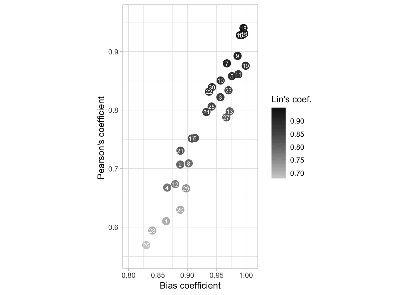

library(cowplot)
theme_set(theme_light())
fig4 <- plot_grid(fig4a, fig4b, align = "hv", ncol = 2, rel_widths = c(1, 1.44), labels = "AUTO")
ggsave("figs/fig4.png", fig4, width = 5.5, dpi = 600)

Hypothesis tests

Here our goal is to compare CCC statistics among the four rating systems. We will assume the raters used in the study constitute a random sample of raters with different abilities for estimating disease severity. We will fit a multi-level (mixed) model using the lme4 package and compare means using the emmeans package.

In the model, the rating systems are fixed effects and raters are random effects. A dummy variable representing unaided and aided assessment was created and added as random effects to account for the dependency because the same raters repeated the assessment based on the different systems.

We need to prepare the data for this analysis. First, let’s reshape the data to wide format so we can fit the model separately for each Lin’s CCC statistics. We will also create the variable with the names of the methods.

ccc2 <- ccc %>%
  filter(stat != "ccc.lower") %>%
  filter(stat != "ccc.upper") %>%
  spread(stat, coef)

ccc2$method2 <- ifelse(ccc2$method == "UN", "UNAIDED", "AIDED")

We want to check whether baseline accuracy influence the results. Let’s create a new data set for the categories or groups of raters according to their baseline accuracy using the case_when function again and the left_join to combine the new data set with the one with all variables.

ccc3 <- ccc2 %>%
  filter(method == "UN") %>%
  mutate(baseline_class = case_when(
    est < 0.8 ~ "Poor",
    est < 0.9 ~ "Fair",
    est < 1 ~ "Good"
  ))
ccc4 <- ccc3 %>% select(rater, baseline_class)
ccc5 <- left_join(ccc2, ccc4, by = "rater")

We need a trick here for ordering the categories how we want them appearing in the plot.

# ordering the factor levels for the plot
ccc5$baseline_class <- factor(ccc5$baseline_class, levels = c("Poor", "Fair", "Good"))

Rename the levels of method variable using revalue function of plyr.

# rename the variables
library(plyr)
ccc5$method <- revalue(ccc5$method, c(
  "estimate_HB" = "HB",
  "estimate_HB2" = "HB2",
  "estimate_LIN" = "LIN",
  "estimate_LIN2" = "LIN2"
))
library(dplyr) # to avoid conflict we reload dplyr

Now we can produce the plot

ccc5 %>%
  ggplot(aes(method, est)) +
  geom_boxplot() +
  facet_wrap(~ baseline_class) +
  labs(x = "Rating system", y = "Lin's CCC") +
   theme_light()+
  theme(axis.text.x = element_text(angle = 0, hjust = 1)) +
  ggsave("figs/fig7.png", width = 7, height = 4)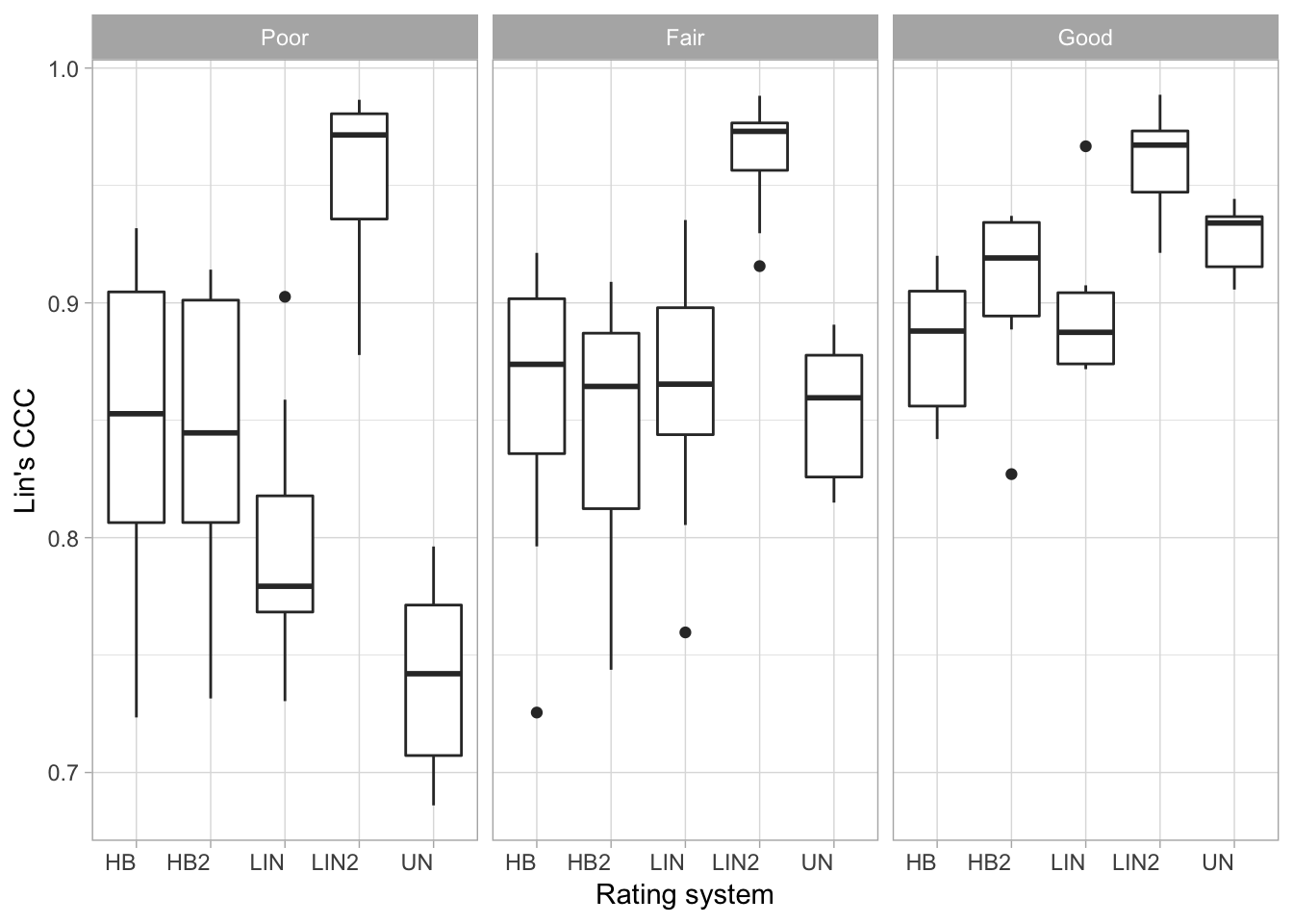

Effect of baseline accuracy on bias coefficient

ccc5 %>%
  ggplot(aes(method, Cb)) +
  geom_boxplot() +
  facet_wrap(~ baseline_class) +
  labs(x = "Rating system", y = "Bias coefficient") +
   theme_light()+
  theme(axis.text.x = element_text(angle = 45, hjust = 1))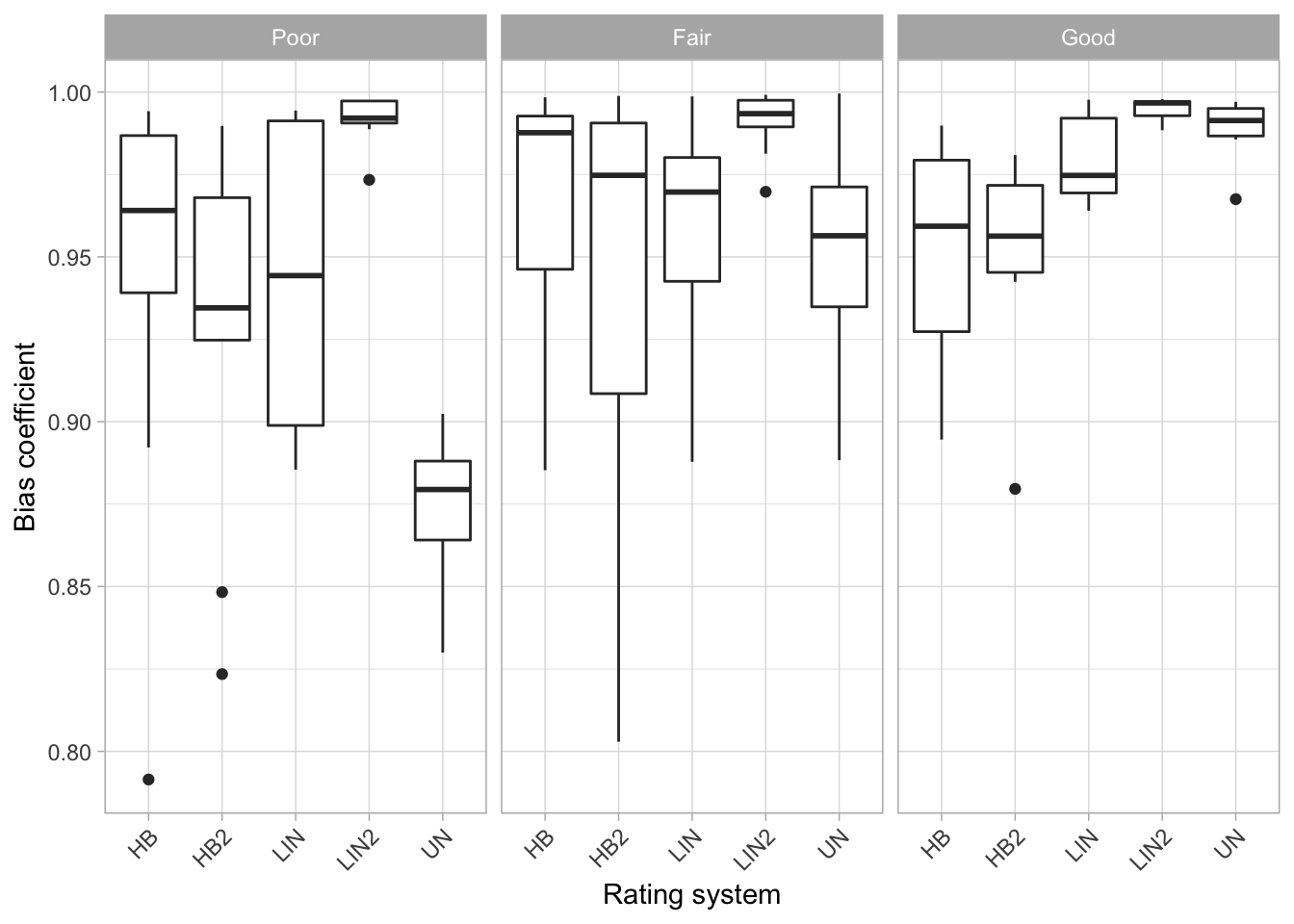

Effect on precision by rater group

ccc5 %>%
  ggplot(aes(method, r)) +
  geom_boxplot() +
   theme_light()+
  facet_wrap(~ baseline_class) +
  labs(x = "Rating system", y = "Person's coefficient") +
  theme(axis.text.x = element_text(angle = 45, hjust = 1))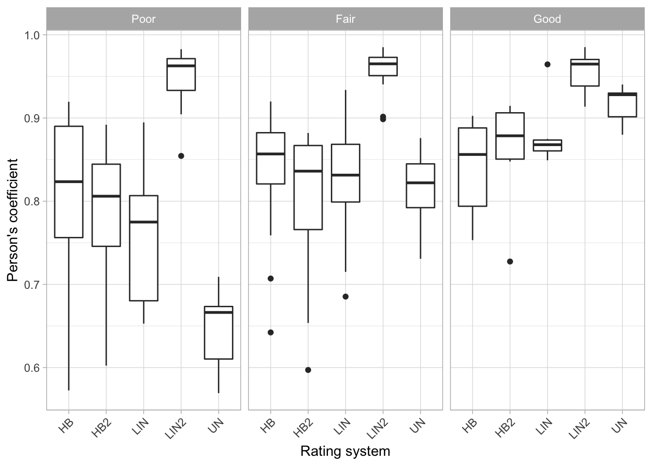

Lin’s CCC

We are now ready to fit the mixed model to Lin’s statistics data.

library(lme4)
mix_pc <- lmer(est ~ method + (1 | rater), data = ccc5)

Summary of the model and significance.

summary(mix_pc)

## Linear mixed model fit by REML ['lmerMod']
## Formula: est ~ method + (1 | rater)
##    Data: ccc5
## 
## REML criterion at convergence: -424.6
## 
## Scaled residuals: 
##     Min      1Q  Median      3Q     Max 
## -2.6430 -0.4639  0.1401  0.5433  1.8694 
## 
## Random effects:
##  Groups   Name        Variance Std.Dev.
##  rater    (Intercept) 0.001038 0.03222 
##  Residual             0.002183 0.04673 
## Number of obs: 150, groups:  rater, 30
## 
## Fixed effects:
##              Estimate Std. Error t value
## (Intercept)  0.860192   0.010362  83.011
## methodHB2   -0.005001   0.012065  -0.414
## methodLIN   -0.009020   0.012065  -0.748
## methodLIN2   0.100431   0.012065   8.324
## methodUN    -0.024524   0.012065  -2.033
## 
## Correlation of Fixed Effects:
##            (Intr) mthHB2 mthLIN mtLIN2
## methodHB2  -0.582                     
## methodLIN  -0.582  0.500              
## methodLIN2 -0.582  0.500  0.500       
## methodUN   -0.582  0.500  0.500  0.500

library(car)
Anova(mix_pc)

Now the lsmeans estimates using emmeans package.

library(emmeans)
mean_pc <- emmeans(mix_pc, ~ method)
df_pc <- cld(mean_pc)
df_pc <- df_pc %>%
  select(method, emmean, .group) %>%
  mutate(stat = "pc")
df_pc

Bias coefficient

# Bc
mix_Cb <- lmer(Cb ~ method + (1 + method2 | rater), data = ccc5)

summary(mix_Cb)

## Linear mixed model fit by REML ['lmerMod']
## Formula: Cb ~ method + (1 + method2 | rater)
##    Data: ccc5
## 
## REML criterion at convergence: -508.4
## 
## Scaled residuals: 
##     Min      1Q  Median      3Q     Max 
## -3.3390 -0.4641  0.0765  0.6188  1.9039 
## 
## Random effects:
##  Groups   Name           Variance  Std.Dev. Corr 
##  rater    (Intercept)    0.0005694 0.02386       
##           method2UNAIDED 0.0012378 0.03518  -0.19
##  Residual                0.0010594 0.03255       
## Number of obs: 150, groups:  rater, 30
## 
## Fixed effects:
##              Estimate Std. Error t value
## (Intercept)  0.956895   0.007369 129.862
## methodHB2   -0.015891   0.008404  -1.891
## methodLIN    0.002197   0.008404   0.261
## methodLIN2   0.035514   0.008404   4.226
## methodUN    -0.022513   0.010578  -2.128
## 
## Correlation of Fixed Effects:
##            (Intr) mthHB2 mthLIN mtLIN2
## methodHB2  -0.570                     
## methodLIN  -0.570  0.500              
## methodLIN2 -0.570  0.500  0.500       
## methodUN   -0.521  0.397  0.397  0.397

mean_Cb <- emmeans(mix_Cb, ~ method)
df_Cb <- cld(mean_Cb)
df_Cb <- df_Cb %>%
  select(method, emmean, .group) %>%
  mutate(stat = "Cb")
df_Cb

Precision

# r
mix_r <- lmer(r ~ method + (1 + method2 | rater), data = ccc5)

summary(mix_r)

## Linear mixed model fit by REML ['lmerMod']
## Formula: r ~ method + (1 + method2 | rater)
##    Data: ccc5
## 
## REML criterion at convergence: -326.3
## 
## Scaled residuals: 
##     Min      1Q  Median      3Q     Max 
## -2.9765 -0.3927  0.1111  0.4950  1.9024 
## 
## Random effects:
##  Groups   Name           Variance Std.Dev. Corr
##  rater    (Intercept)    0.002040 0.04517      
##           method2UNAIDED 0.005287 0.07271  0.10
##  Residual                0.003536 0.05947      
## Number of obs: 150, groups:  rater, 30
## 
## Fixed effects:
##             Estimate Std. Error t value
## (Intercept)  0.82499    0.01363  60.510
## methodHB2   -0.01814    0.01535  -1.181
## methodLIN   -0.00733    0.01535  -0.477
## methodLIN2   0.12846    0.01535   8.367
## methodUN    -0.04091    0.02030  -2.016
## 
## Correlation of Fixed Effects:
##            (Intr) mthHB2 mthLIN mtLIN2
## methodHB2  -0.563                     
## methodLIN  -0.563  0.500              
## methodLIN2 -0.563  0.500  0.500       
## methodUN   -0.385  0.378  0.378  0.378

mean_r <- emmeans(mix_r, ~ method)
df_r <- cld(mean_r)
df_r <- df_r %>%
  select(method, emmean, .group) %>%
  mutate(stat = "r")

location-shift

# l.shift
mix_l.shift <- lmer(l.shift ~ method + (1 + method2 | rater), data = ccc5)
summary(mix_l.shift)

## Linear mixed model fit by REML ['lmerMod']
## Formula: l.shift ~ method + (1 + method2 | rater)
##    Data: ccc5
## 
## REML criterion at convergence: -119.4
## 
## Scaled residuals: 
##      Min       1Q   Median       3Q      Max 
## -2.32082 -0.48522 -0.05746  0.58141  2.14714 
## 
## Random effects:
##  Groups   Name           Variance Std.Dev. Corr
##  rater    (Intercept)    0.01997  0.1413       
##           method2UNAIDED 0.04782  0.2187   0.53
##  Residual                0.01089  0.1044       
## Number of obs: 150, groups:  rater, 30
## 
## Fixed effects:
##             Estimate Std. Error t value
## (Intercept)  0.14943    0.03208   4.659
## methodHB2    0.14517    0.02695   5.387
## methodLIN   -0.01241    0.02695  -0.460
## methodLIN2  -0.15975    0.02695  -5.928
## methodUN    -0.08140    0.04817  -1.690
## 
## Correlation of Fixed Effects:
##            (Intr) mthHB2 mthLIN mtLIN2
## methodHB2  -0.420                     
## methodLIN  -0.420  0.500              
## methodLIN2 -0.420  0.500  0.500       
## methodUN    0.119  0.280  0.280  0.280

mean_l.shift <- emmeans(mix_l.shift, ~ method)
df_l.shift <- cld(mean_l.shift)
df_l.shift <- df_l.shift %>%
  select(method, emmean, .group) %>%
  mutate(stat = "l.shift")

Scale-shift

mix_s.shift <- lmer(s.shift ~ method + (1 + method2 | rater), data = ccc5)
summary(mix_s.shift)

## Linear mixed model fit by REML ['lmerMod']
## Formula: s.shift ~ method + (1 + method2 | rater)
##    Data: ccc5
## 
## REML criterion at convergence: -250.3
## 
## Scaled residuals: 
##     Min      1Q  Median      3Q     Max 
## -3.2195 -0.4817 -0.0041  0.5169  2.5209 
## 
## Random effects:
##  Groups   Name           Variance Std.Dev. Corr
##  rater    (Intercept)    0.006506 0.08066      
##           method2UNAIDED 0.008903 0.09436  0.72
##  Residual                0.005435 0.07373      
## Number of obs: 150, groups:  rater, 30
## 
## Fixed effects:
##             Estimate Std. Error t value
## (Intercept)  1.17005    0.01995  58.646
## methodHB2   -0.05234    0.01904  -2.749
## methodLIN   -0.21892    0.01904 -11.501
## methodLIN2  -0.22489    0.01904 -11.814
## methodUN    -0.18671    0.02567  -7.272
## 
## Correlation of Fixed Effects:
##            (Intr) mthHB2 mthLIN mtLIN2
## methodHB2  -0.477                     
## methodLIN  -0.477  0.500              
## methodLIN2 -0.477  0.500  0.500       
## methodUN    0.004  0.371  0.371  0.371

mean_s.shift <- emmeans(mix_s.shift, ~ method)
df_s.shift <- cld(mean_s.shift)
df_s.shift <- df_s.shift %>%
  select(method, emmean, .group) %>%
  mutate(stat = "s.shift")

CCC summary

We will combine all statistics and produce a table with the results including the means separation test.

df_all <- rbind(df_pc, df_r, df_Cb, df_s.shift, df_l.shift) %>%
  mutate(emmean = round(as.numeric(emmean), 2))


table1 <- df_all %>%
  unite(emmean2, emmean, .group, sep = " ") %>%
  spread(stat, emmean2)

library(knitr)
kable(table1)

method	Cb	l.shift	pc	r	s.shift
HB	0.96 1	0.15 2	0.86 1	0.82 1	1.17 2
HB2	0.94 1	0.29 3	0.86 1	0.81 1	1.12 2
LIN	0.96 1	0.14 2	0.85 1	0.82 1	0.95 1
LIN2	0.99 2	-0.01 1	0.96 2	0.95 2	0.95 1
UN	0.93 1	0.07 12	0.84 1	0.78 1	0.98 1

Effect of baseline accuracy

Here we want to check whether the effect of the aid was affected by the baseline accuracy of the raters, split into different groups.

# pc
ccc6 <- ccc5 %>%
  filter(method != "UN")

mix_pc_base <- lmer(est ~ method * baseline_class + (1 | rater), data = ccc6)
summary(mix_pc_base)

## Linear mixed model fit by REML ['lmerMod']
## Formula: est ~ method * baseline_class + (1 | rater)
##    Data: ccc6
## 
## REML criterion at convergence: -338.1
## 
## Scaled residuals: 
##     Min      1Q  Median      3Q     Max 
## -2.5115 -0.4794  0.1146  0.4690  1.9257 
## 
## Random effects:
##  Groups   Name        Variance  Std.Dev.
##  rater    (Intercept) 0.0007011 0.02648 
##  Residual             0.0015411 0.03926 
## Number of obs: 120, groups:  rater, 30
## 
## Fixed effects:
##                                Estimate Std. Error t value
## (Intercept)                    0.845812   0.015784  53.587
## methodHB2                     -0.002040   0.018506  -0.110
## methodLIN                     -0.046039   0.018506  -2.488
## methodLIN2                     0.108455   0.018506   5.861
## baseline_classFair             0.014145   0.019965   0.708
## baseline_classGood             0.036536   0.024957   1.464
## methodHB2:baseline_classFair  -0.015654   0.023408  -0.669
## methodLIN:baseline_classFair   0.049038   0.023408   2.095
## methodLIN2:baseline_classFair -0.003728   0.023408  -0.159
## methodHB2:baseline_classGood   0.024331   0.029260   0.832
## methodLIN:baseline_classGood   0.062498   0.029260   2.136
## methodLIN2:baseline_classGood -0.030800   0.029260  -1.053
## 
## Correlation of Fixed Effects:
##             (Intr) mthHB2 mthLIN mtLIN2 bsln_F bsln_G
## methodHB2   -0.586                                   
## methodLIN   -0.586  0.500                            
## methodLIN2  -0.586  0.500  0.500                     
## bsln_clssFr -0.791  0.463  0.463  0.463              
## bsln_clssGd -0.632  0.371  0.371  0.371  0.500       
## mthdHB2:b_F  0.463 -0.791 -0.395 -0.395 -0.586 -0.293
## mthdLIN:b_F  0.463 -0.395 -0.791 -0.395 -0.586 -0.293
## mthdLIN2:_F  0.463 -0.395 -0.395 -0.791 -0.586 -0.293
## mthdHB2:b_G  0.371 -0.632 -0.316 -0.316 -0.293 -0.586
## mthdLIN:b_G  0.371 -0.316 -0.632 -0.316 -0.293 -0.586
## mthdLIN2:_G  0.371 -0.316 -0.316 -0.632 -0.293 -0.586
##             mHB2:_F mLIN:_F mLIN2:_F mHB2:_G mLIN:_G
## methodHB2                                           
## methodLIN                                           
## methodLIN2                                          
## bsln_clssFr                                         
## bsln_clssGd                                         
## mthdHB2:b_F                                         
## mthdLIN:b_F  0.500                                  
## mthdLIN2:_F  0.500   0.500                          
## mthdHB2:b_G  0.500   0.250   0.250                  
## mthdLIN:b_G  0.250   0.500   0.250    0.500         
## mthdLIN2:_G  0.250   0.250   0.500    0.500   0.500

Anova(mix_pc_base)

mean_pc_base <- emmeans(mix_pc_base, ~ method * baseline_class)
df_pc_base <- cld(mean_pc_base)
df_pc_base <- df_pc_base %>%
  select(method, baseline_class, emmean, .group) %>%
  mutate(stat = "pc")
df_pc_base

mix_cb_base <- lmer(Cb ~ method * baseline_class + (1 | rater), data = ccc6)

summary(mix_cb_base)

## Linear mixed model fit by REML ['lmerMod']
## Formula: Cb ~ method * baseline_class + (1 | rater)
##    Data: ccc6
## 
## REML criterion at convergence: -373
## 
## Scaled residuals: 
##     Min      1Q  Median      3Q     Max 
## -3.3772 -0.4748  0.0769  0.6050  1.6607 
## 
## Random effects:
##  Groups   Name        Variance  Std.Dev.
##  rater    (Intercept) 0.0005795 0.02407 
##  Residual             0.0010858 0.03295 
## Number of obs: 120, groups:  rater, 30
## 
## Fixed effects:
##                                Estimate Std. Error t value
## (Intercept)                    0.944419   0.013603  69.428
## methodHB2                     -0.015968   0.015534  -1.028
## methodLIN                      0.002106   0.015534   0.136
## methodLIN2                     0.047186   0.015534   3.038
## baseline_classFair             0.022342   0.017207   1.298
## baseline_classGood             0.006526   0.021508   0.303
## methodHB2:baseline_classFair  -0.005293   0.019649  -0.269
## methodLIN:baseline_classFair  -0.010366   0.019649  -0.528
## methodLIN2:baseline_classFair -0.021989   0.019649  -1.119
## methodHB2:baseline_classGood   0.013618   0.024561   0.554
## methodLIN:baseline_classGood   0.026373   0.024561   1.074
## methodLIN2:baseline_classGood -0.003386   0.024561  -0.138
## 
## Correlation of Fixed Effects:
##             (Intr) mthHB2 mthLIN mtLIN2 bsln_F bsln_G
## methodHB2   -0.571                                   
## methodLIN   -0.571  0.500                            
## methodLIN2  -0.571  0.500  0.500                     
## bsln_clssFr -0.791  0.451  0.451  0.451              
## bsln_clssGd -0.632  0.361  0.361  0.361  0.500       
## mthdHB2:b_F  0.451 -0.791 -0.395 -0.395 -0.571 -0.285
## mthdLIN:b_F  0.451 -0.395 -0.791 -0.395 -0.571 -0.285
## mthdLIN2:_F  0.451 -0.395 -0.395 -0.791 -0.571 -0.285
## mthdHB2:b_G  0.361 -0.632 -0.316 -0.316 -0.285 -0.571
## mthdLIN:b_G  0.361 -0.316 -0.632 -0.316 -0.285 -0.571
## mthdLIN2:_G  0.361 -0.316 -0.316 -0.632 -0.285 -0.571
##             mHB2:_F mLIN:_F mLIN2:_F mHB2:_G mLIN:_G
## methodHB2                                           
## methodLIN                                           
## methodLIN2                                          
## bsln_clssFr                                         
## bsln_clssGd                                         
## mthdHB2:b_F                                         
## mthdLIN:b_F  0.500                                  
## mthdLIN2:_F  0.500   0.500                          
## mthdHB2:b_G  0.500   0.250   0.250                  
## mthdLIN:b_G  0.250   0.500   0.250    0.500         
## mthdLIN2:_G  0.250   0.250   0.500    0.500   0.500

Anova(mix_cb_base)

mean_cb <- emmeans(mix_cb_base, ~ method * baseline_class)
df_cb <- cld(mean_cb)
df_cb <- df_cb %>%
  select(method, baseline_class, emmean, .group) %>%
  mutate(stat = "cb")
df_cb

# pc
ccc6 <- ccc5 %>%
  filter(method != "UN")

mix_r_base <- lmer(r ~ method * baseline_class + (1 | rater), data = ccc6)
summary(mix_r_base)

## Linear mixed model fit by REML ['lmerMod']
## Formula: r ~ method * baseline_class + (1 | rater)
##    Data: ccc6
## 
## REML criterion at convergence: -249.9
## 
## Scaled residuals: 
##      Min       1Q   Median       3Q      Max 
## -2.85965 -0.33467  0.07567  0.62742  1.79889 
## 
## Random effects:
##  Groups   Name        Variance Std.Dev.
##  rater    (Intercept) 0.001789 0.04230 
##  Residual             0.003403 0.05833 
## Number of obs: 120, groups:  rater, 30
## 
## Fixed effects:
##                               Estimate Std. Error t value
## (Intercept)                    0.80199    0.02402  33.391
## methodHB2                     -0.01612    0.02750  -0.586
## methodLIN                     -0.04362    0.02750  -1.586
## methodLIN2                     0.14444    0.02750   5.253
## baseline_classFair             0.03080    0.03038   1.014
## baseline_classGood             0.03801    0.03798   1.001
## methodHB2:baseline_classFair  -0.01821    0.03478  -0.524
## methodLIN:baseline_classFair   0.03895    0.03478   1.120
## methodLIN2:baseline_classFair -0.02019    0.03478  -0.580
## methodHB2:baseline_classGood   0.03545    0.04348   0.815
## methodLIN:baseline_classGood   0.08408    0.04348   1.934
## methodLIN2:baseline_classGood -0.02943    0.04348  -0.677
## 
## Correlation of Fixed Effects:
##             (Intr) mthHB2 mthLIN mtLIN2 bsln_F bsln_G
## methodHB2   -0.572                                   
## methodLIN   -0.572  0.500                            
## methodLIN2  -0.572  0.500  0.500                     
## bsln_clssFr -0.791  0.453  0.453  0.453              
## bsln_clssGd -0.632  0.362  0.362  0.362  0.500       
## mthdHB2:b_F  0.453 -0.791 -0.395 -0.395 -0.572 -0.286
## mthdLIN:b_F  0.453 -0.395 -0.791 -0.395 -0.572 -0.286
## mthdLIN2:_F  0.453 -0.395 -0.395 -0.791 -0.572 -0.286
## mthdHB2:b_G  0.362 -0.632 -0.316 -0.316 -0.286 -0.572
## mthdLIN:b_G  0.362 -0.316 -0.632 -0.316 -0.286 -0.572
## mthdLIN2:_G  0.362 -0.316 -0.316 -0.632 -0.286 -0.572
##             mHB2:_F mLIN:_F mLIN2:_F mHB2:_G mLIN:_G
## methodHB2                                           
## methodLIN                                           
## methodLIN2                                          
## bsln_clssFr                                         
## bsln_clssGd                                         
## mthdHB2:b_F                                         
## mthdLIN:b_F  0.500                                  
## mthdLIN2:_F  0.500   0.500                          
## mthdHB2:b_G  0.500   0.250   0.250                  
## mthdLIN:b_G  0.250   0.500   0.250    0.500         
## mthdLIN2:_G  0.250   0.250   0.500    0.500   0.500

Anova(mix_r_base)

mean_r_base <- emmeans(mix_r_base, ~ method * baseline_class)
df_r_base <- cld(mean_r_base)
df_r_base <- df_r_base %>%
  select(method, baseline_class, emmean, .group) %>%
  mutate(stat = "r")
df_r_base

Interrater reliability

Two methods will be used here. The overall concordance coefficient and the intra-class correlation coefficient.

UN

library(irr)
library(rel)

sad_UN <- dat_cls %>%
  select(rater, UN) %>%
  group_by(rater) %>%
  mutate(id = 1:n()) %>%
  spread(rater, UN) %>%
  select(2:31) %>%
  data.matrix()
sad_occc_UN <- epi.occc(sad_UN, na.rm = FALSE, pairs = TRUE)
sad_icc_UN <- icc(sad_UN, model = "two", measure = "single", type = "agreement")
sad_occc_UN$occc

## [1] 0.7431051

sad_icc_UN$est

##     Const 
## 0.7470855

LIN

sad_estimate_LIN <- dat_cls %>%
  select(rater, LIN) %>%
  group_by(rater) %>%
  mutate(id = 1:n()) %>%
  spread(rater, LIN) %>%
  select(2:31) %>%
  data.matrix()
sad_occc_estimate_LIN <- epi.occc(sad_estimate_LIN, na.rm = FALSE, pairs = TRUE)
sad_icc_estimate_LIN <- icc(sad_estimate_LIN, model = "two", measure = "single", type = "agreement")
sad_occc_estimate_LIN$occc

## [1] 0.8144513

sad_icc_estimate_LIN$est

##     Const 
## 0.8182493

LOG

sad_estimate_HB2 <- dat_cls %>%
  select(rater, HB2) %>%
  group_by(rater) %>%
  mutate(id = 1:n()) %>%
  spread(rater, HB2) %>%
  select(2:31) %>%
  data.matrix()
sad_occc_estimate_HB2 <- epi.occc(sad_estimate_HB2, na.rm = FALSE, pairs = TRUE)
library(rel)
sad_icc_estimate_HB2 <- icc(sad_estimate_HB2, model = "two", measure = "single", type = "agreement")
sad_occc_estimate_HB2$occc

## [1] 0.8353876

sad_icc_estimate_HB2$est

##     Const 
## 0.8392391

LIN2

sad_estimate_LIN2 <- dat_cls %>%
  select(rater, LIN2) %>%
  group_by(rater) %>%
  mutate(id = 1:n()) %>%
  spread(rater, LIN2) %>%
  select(2:31) %>%
  data.matrix()
sad_occc_estimate_LIN2 <- epi.occc(sad_estimate_LIN2, na.rm = FALSE, pairs = TRUE)
sad_icc_estimate_LIN2 <- icc(sad_estimate_LIN2, model = "two", measure = "single", type = "agreement")
sad_occc_estimate_LIN2$occc

## [1] 0.9298292

sad_icc_estimate_LIN2$est

##     Const 
## 0.9317496

LOG2

sad_estimate_HB <- dat_cls %>%
  select(rater, HB) %>%
  group_by(rater) %>%
  mutate(id = 1:n()) %>%
  spread(rater, HB) %>%
  select(2:31) %>%
  data.matrix()
sad_occc_estimate_HB <- epi.occc(sad_estimate_HB, na.rm = FALSE, pairs = TRUE)
sad_icc_estimate_HB <- icc(sad_estimate_HB, model = "two", measure = "single", type = "agreement")
sad_occc_estimate_HB$occc

## [1] 0.8202141

sad_icc_estimate_HB$est

##     Const 
## 0.8242236

Summary

Here is a summary table with the inter-rater reliability or reproducibility results.

Method <- c("sad_UN", "sad_estimate_LIN2", "sad_estimate_LIN", "sad_estimate_HB2", "sad_estimate_HB")

OCCC <- c(sad_occc_UN$occc, sad_occc_estimate_LIN2$occc, sad_occc_estimate_LIN$occc, sad_occc_estimate_HB2$occc, sad_occc_estimate_HB$occc)

ICC <- c(sad_icc_UN$est, sad_icc_estimate_LIN2$est, sad_icc_estimate_LIN$est, sad_icc_estimate_HB2$est, sad_icc_estimate_HB$est)

ICC_l <- c(sad_icc_UN$lb, sad_icc_estimate_LIN2$lb, sad_icc_estimate_LIN$lb, sad_icc_estimate_HB2$lb, sad_icc_estimate_HB$lb)


ICC_u <- c(sad_icc_UN$ub, sad_icc_estimate_LIN2$ub, sad_icc_estimate_LIN$ub, sad_icc_estimate_HB2$ub, sad_icc_estimate_HB$ub)

table2 <- data.frame(Method, OCCC, ICC, ICC_l, ICC_u)
table2

Developed by Emerson Del Ponte.