Fit Gradient Models to Data

This function fits three gradient models (exponential, power, and modified power) to given data. It then ranks the models based on their R-squared values and returns diagnostic plots for each model.

Usage

fit_gradients(data, C = 1)

Arguments

data

A dataframe containing the data, with columns "x" representing distances and "Y" representing the corresponding measurements or counts.

C

A constant to be used in the modified power model. Defaults to 1.

Value

A list containing:

• dataThe input data, which will include an additional column 'mod_x'.

• results_tableA table of the model parameters and R-squared values.

• plot_exponentialDiagnostic plot for the exponential model.

• plot_powerDiagnostic plot for the power model.

• plot_modified_powerDiagnostic plot for the modified power model.

• plot_exponential_originalPlot of the original data with the exponential model fit.

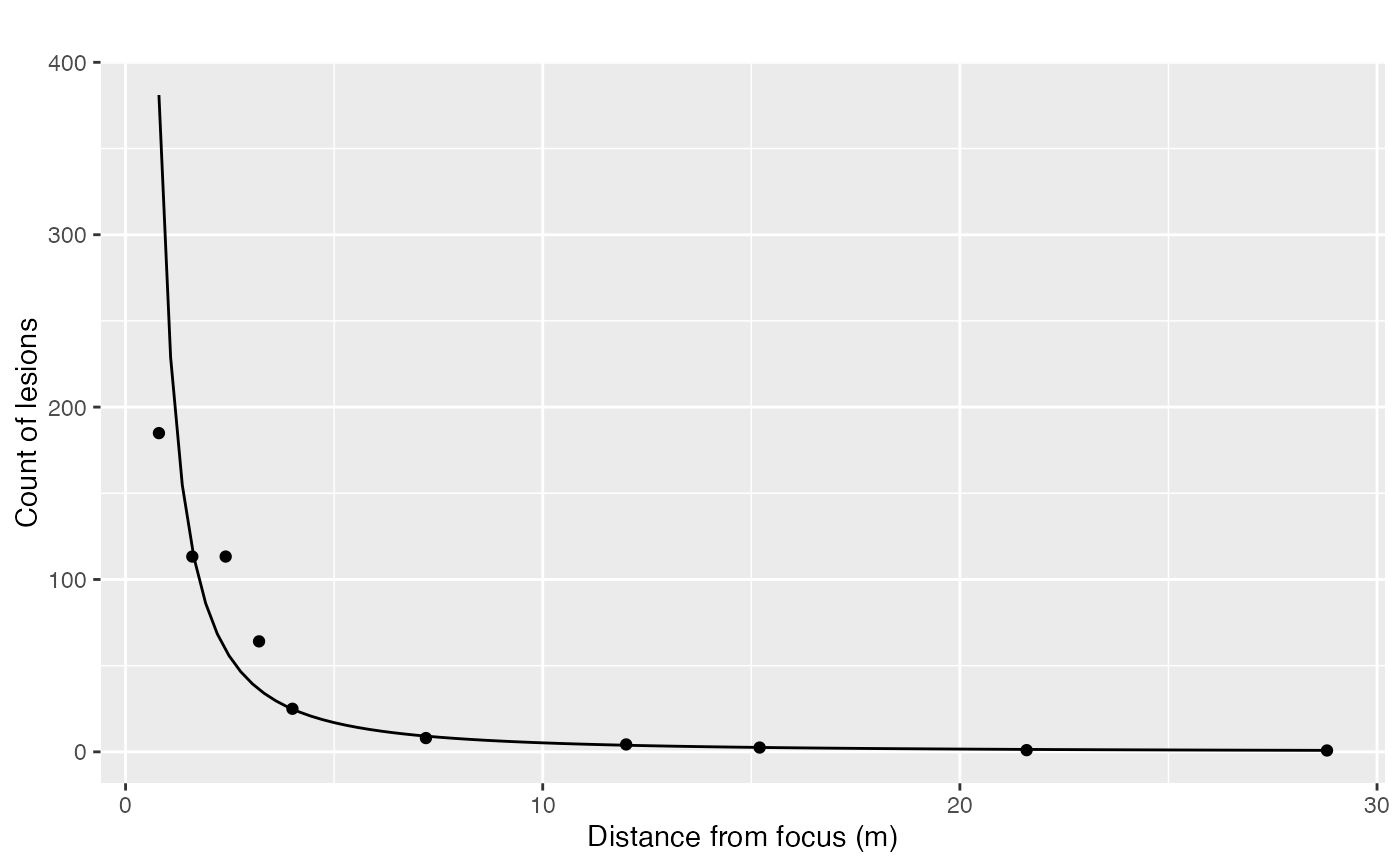
• plot_power_originalPlot of the original data with the power model fit.

• plot_modified_power_originalPlot of the original data with the modified power model fit.

Examples

x <- c(0.8, 1.6, 2.4, 3.2, 4, 7.2, 12, 15.2, 21.6, 28.8)
Y <- c(184.9, 113.3, 113.3, 64.1, 25, 8, 4.3, 2.5, 1, 0.8)
grad1 <- data.frame(x = x, Y = Y)
library(ggplot2)
mg <- fit_gradients(grad1, C = 0.4)
mg$plot_power_original +
  labs(title = "", x = "Distance from focus (m)", y = "Count of lesions")